What your professor was pointing at
Andrew, I like this one, and I think your professor was right to get animated. You already know the sentence everyone repeats: without those operations the layers collapse into one. Yours is the better question: why does that deserve the excitement? My short answer is that the bend does not switch learning on. A straight-line model learns perfectly well, and anyone who said otherwise was compressing too hard. What the bend changes is what the model is able to learn at all, and that is the whole ball game.
So the answer has two halves, and keeping them apart is most of the work. The first half is representation: which relationships the model can express, before any training happens. The second half is learning: how training searches inside whatever the model can express. Your professor's excitement was about the first half, because it is the one that no amount of data, patience or compute can fix. The representation argument comes first, with four points and one fold, and then a complete learning step through a fold by hand, every number on the page.
Two linear layers are one linear layer
Start with what a layer is. A linear layer takes a list of numbers, a vector, and multiplies it by a grid of numbers called a matrix. The whole operation in two dimensions is small enough to check by hand. Take the matrix $\mathbf{W}_1$ acting on the input $\mathbf{x}$:
$$\mathbf{W}_1 = \begin{bmatrix} 2 & 0 \\ 1 & 1 \end{bmatrix}, \qquad \mathbf{x} = \begin{bmatrix} 1 \\ 1 \end{bmatrix}, \qquad \mathbf{W}_1\mathbf{x} = \begin{bmatrix} 2\cdot 1 + 0 \cdot 1 \\ 1 \cdot 1 + 1 \cdot 1\end{bmatrix} = \begin{bmatrix} 2 \\ 2 \end{bmatrix}$$In words: each row of the matrix is paired with the input list, multiplied across position by position, and added up to make one number of the output. Two rows, so two output numbers. That is the entire arithmetic of a linear layer, repeated at industrial scale.
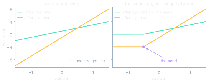
Now stack a second one on top, which is what two layers in a row do to your numbers. The key fact is that you can multiply the two matrices together first and get a single matrix that does the same job:
$$\mathbf{W}_2 = \begin{bmatrix} 1 & 1 \\ 0 & 1 \end{bmatrix}, \qquad \mathbf{W}_2\mathbf{W}_1 = \begin{bmatrix} 3 & 1 \\ 1 & 1 \end{bmatrix}$$In words: each entry comes from a row of the second grid paired with a column of the first, because the second map is the one applied last, and the result is one grid. Check it on our input: the first layer sent the vector one-one to two-two, and the second sends two-two to four-two. The combined grid sends one-one straight to four-two in a single step.
The same collapse happens with the offsets that real layers add. A multiply-then-add followed by another multiply-then-add is still one multiply-then-add. And it does not stop at two: ten of these in a row, or a hundred, and the same multiplication eats the entire stack. Depth built from linear layers alone buys no new kinds of answer. It buys a slower way to compute an answer the single layer already had.
The four points a line cannot split
Now a job that stack cannot do, small enough to hold in your head. Two switches, each off or on, which gives four settings in total. We want an output of one when exactly one switch is on, and zero when the two switches agree. Engineers call the rule exclusive or, and it is the standard counterexample.
Draw the four settings as four points on a square and try to separate them with one straight cut. Tilt it, slide it, and one point is always stranded on the wrong side. This is not a training problem you could fix with more data, and there is a two-line proof.
Any straight cut that puts two points on the same side must also put the midpoint of those two points on that side, because a straight boundary cannot let a segment leave and come back. The two settings that want a one are the corners at one-zero and zero-one, and their midpoint is the center of the square. The two that want a zero are zero-zero and one-one, and their midpoint is also the center of the square. So the center would have to be on both sides at once, and no straight cut exists.
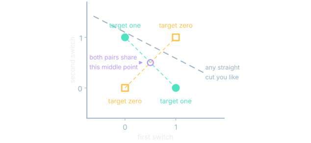
This is the shape of your professor's excitement. When a model family is missing an answer, training is not slow. It is impossible, in a way that has nothing to do with the data.
One hinge changes the space
The fix is one operation, and it is almost too plain to look important. ReLU stands for rectified linear unit. I will call it a hinge, because that is what it looks like. It takes a number, keeps it if it is positive, and replaces it with zero if it is not.
$$\operatorname{ReLU}(z) = \max(0,\, z)$$In words: ReLU of a number is the larger of zero and that number. Its graph is two straight pieces with a single bend where they meet at the origin, so "nonlinear" here does not mean a smooth curve. One bend is enough to break the collapse, because you cannot multiply two grids through a bend.
Now build two small detectors out of it. The first asks how much the first switch beats the second; the second asks the reverse. Call their outputs $h_1$ and $h_2$. Those new numbers are the network's features, its own coordinates for the problem. Let the prediction be their sum:
$$h_1 = \operatorname{ReLU}(x_1 - x_2), \qquad h_2 = \operatorname{ReLU}(x_2 - x_1), \qquad \hat{y} = h_1 + h_2$$In words: subtract the second input from the first and keep only a positive result; do the mirror image for the second detector; then add the two results to get the prediction. Where the two inputs are equal, both detectors report zero.
| Input $(x_1, x_2)$ | $h_1$ | $h_2$ | $\hat{y} = h_1 + h_2$ | Target |
|---|---|---|---|---|
| (0, 0) | 0 | 0 | 0 | 0 |
| (1, 0) | 1 | 0 | 1 | 1 |
| (0, 1) | 0 | 1 | 1 | 1 |
| (1, 1) | 0 | 0 | 0 | 0 |
Compare the sum against a threshold of 0.5 and all four are right. The threshold is not the interesting part. In the new pair of coordinates, the two settings where the switches agree both produce zero and zero, so they land on the same spot, while the other two land one unit out along their own directions. The four points were rearranged, and in their new arrangement a straight line is enough.
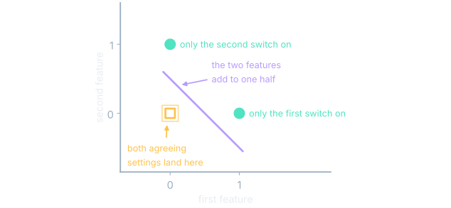
That is the sentence I would put on the board. A network's last step is nearly always something straightforward, a straight cut or a set of scores, and the layers before it exist to hand that step a space in which straightforward is enough. Folding builds the new space, and a stack of grids can never fold.
Representable is not the same as learnable
One caveat about what that demonstration proved. I chose those two detectors myself, knowing the answer in advance, so all it shows is that the architecture can express a solution. Whether training would find one is a separate question.
So what does training have to find? The hinge rule never changes, so what moves are the weights around it. The weight feeding a hinge sets how steep its ramp is and which side is flat; the offset added before the hinge sets where along the input the bend sits; the weight after it sets how much that unit contributes to the answer. A hinge is a fold whose position, angle and depth are all learned.
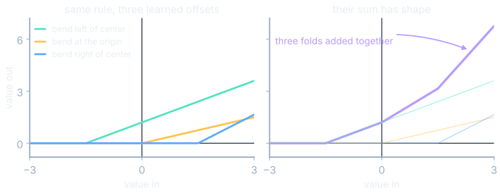
With enough folds a network can follow almost any shape you care to name. That result is called universal approximation, and it promises one thing: that a setting of the weights exists. It says nothing about whether training reaches it, or whether the result works on anything outside the data you had.
A complete learning step, through the hinge
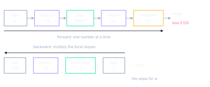
Now the other half, on the smallest network that still has a fold in it. One input $x = 2$; one weight $w$ before the hinge; one weight $v$ after it; no offsets; both weights starting at 0.5; the target $t = 1$.
Forward: what the network says
The input meets the first weight, the product goes into the hinge, and the hinge output meets the second weight to make the prediction $\hat{y}$:
$$h = \operatorname{ReLU}(w x) = \operatorname{ReLU}(0.5 \cdot 2) = 1, \qquad \hat{y} = v h = 0.5 \cdot 1 = 0.5$$We landed on the live side of the fold, where the ramp is, so the hinge passed its input through untouched. Now score the guess. The loss squares the gap, which makes it positive and punishes big misses harder, and then halves it so the arithmetic downstream comes out clean:
$$L = \tfrac{1}{2}(\hat{y} - t)^2 = \tfrac{1}{2}(0.5 - 1)^2 = \tfrac{1}{2}(0.25) = 0.125$$In words: the prediction is half of what it should be, the gap is minus one half, squaring gives a quarter, and halving that gives an eighth. That eighth is the number the next few steps exist to shrink.
To shrink it we need to know which way to move each weight, and that is what a gradient is: an arrow pointing the way that makes the loss grow fastest. Training reads that arrow and walks the other way.
For a weight buried behind a hinge, we get the arrow from the chain rule: walk the path from the loss back to the weight and multiply the local rates of change you meet. That walk, done for every weight at once, is what people call backpropagation.
Backward: two slopes, four factors
The weight after the fold has the shorter path. Two factors reach it: the gap at the output, and the value that weight was multiplying.
$$\frac{\partial L}{\partial v} = (\hat{y} - t)\, h = (-0.5)(1) = -0.5$$The weight in front of the fold has a longer path, and the hinge sits on it. Because we are on the ramp side, a small nudge going in produces the same nudge coming out, so the hinge contributes a factor of one:
$$\frac{\partial L}{\partial w} = (\hat{y} - t)\, v \, \operatorname{ReLU}'(wx)\, x = (-0.5)(0.5)(1)(2) = -0.5$$In words: multiply the gap of minus one half by the second weight of one half, by the hinge's local slope of one, by the input of two. Both weights have a slope of minus one half, and the negative sign says the same thing in both cases: this loss goes down if this weight goes up.
The step, and the payoff
Take a step of one tenth against each slope. That fraction is the learning rate, and both slopes are computed at the old weights before either weight moves.
$$w_{\text{new}} = 0.5 - 0.1(-0.5) = 0.55, \qquad v_{\text{new}} = 0.5 - 0.1(-0.5) = 0.55$$Now run the network forward again with the new weights and score it again:
$$h = \operatorname{ReLU}(0.55 \cdot 2) = 1.1, \quad \hat{y} = 0.55 \cdot 1.1 = 0.605, \quad L = \tfrac{1}{2}(0.605 - 1)^2 = 0.0780$$In words: subtracting a negative amount adds, so both weights rise to 0.55. The prediction moves from 0.5 up to 0.605, the gap shrinks from a half to about four tenths, and the loss falls from 0.125 to 0.078, a little under half its height. That is one complete learning step, with a fold in the middle of it and nothing hidden.
See it move
What the hinge does to the gradient
Everything above used a factor of one at the hinge, which we got for free by landing on the ramp. On the flat side the local slope is zero instead, and a zero multiplied into that chain wipes out every factor behind it: the weight in front receives no instruction at all from that example. The hinge gates the flow of blame as well as the flow of numbers.
That is mostly a feature: each example only adjusts the units that were involved in producing it. But it has a failure mode. If a unit sits on its flat side for every example it ever sees, it never receives a gradient again and never comes back. That is a dead unit, and it is the price the plain hinge charges for being so cheap everywhere else.
The common fix rounds off the corner. Smoothed relatives such as GELU, which chat models use, and SiLU hug the same shape far out on either side but curve gently through the middle, so the quiet side passes back a small rate instead of nothing and a sleeping unit can be woken. Smoothness is not a cure for everything, and plenty of trained networks still use the plain sharp hinge.
Fixed bend, moving weights
The division of labor is short. The hinge is fixed: no parameters, no gradient, identical in every network that uses it. The weights around it are what training moves. Nothing is learned inside the bend, and everything a straight line could not learn is learnable because the bend is there.
Two extensions. A transformer has other nonlinear operations besides the hinge between its feed-forward layers: attention's softmax is one, the normalization steps another. And the folds are one ingredient among several: initialization, residual connections, the optimizer and the data all decide whether a deep network trains at all. The bend makes the good answer reachable; it does not make it easy to reach.
Nonlinear is not random
One last myth, because the word nonlinear sounds like it should mean unpredictable, which is the guess I made myself when I first met it.
Non-straight and unpredictable are different words. The fold is predictable, and what it buys is shape.
What you now know
- Two linear layers in a row multiply out to a single grid, so depth built from linear layers alone adds parameters without adding one new kind of answer.
- Four points defeat every straight cut there is, and the midpoint argument proves it in two lines: a model family can be missing an answer in a way no amount of training repairs.
- One hinge rebuilds the space: two ReLU features send the two agreeing settings to the same spot and leave the other two apart, after which a straight cut at a threshold of 0.5 gets all four right.
- Being able to represent an answer is not the same as finding it; the hand-chosen features prove capacity, and training still has to roll downhill to something as good.
- The buried weight's slope is four multiplications (the gap, the weight after the fold, the hinge's local slope and the input), and one complete step moves the loss from 0.125 to 0.078 as both weights move from 0.5 to 0.55, with the hinge contributing a local slope of one on its live side.
- On its flat side the hinge contributes a zero instead, which gates the blame and can leave a unit dead; the smoothed relatives like GELU round that corner off.
- The bend itself never learns, because it has no parameters at all, and everything a straight line could not learn is learnable because the bend is there.
Where we're headed
Andrew, if I had one sentence for your professor it would be this: the nonlinear operations are what let a network stop merely combining the numbers it was given and start manufacturing better numbers to combine. Four points and one fold is the smallest example, and everything larger is this with more of everything: more folds, more dimensions, more layers handing better coordinates forward. For the folding unit taken apart slowly on its own, there is the neuron chapter in the machine learning book. And if the word nonlinear still carries a whiff of randomness, the first question here shows where the chance in a language model lives.