Projections and Shadows

You have already seen a thousand of these

Open any paper about embeddings and somewhere in it there is a scatter plot: a few hundred colored dots on a flat pair of axes, with clusters labeled "sports," "medicine," "recipes." It is the picture everyone reaches for, and it is genuinely useful.

The previous chapter just told us those dots live in 1000 dimensions. So the plot is not the space. It is a shadow of the space, cast onto a page — and a shadow is a real measurement with real rules about what it can and cannot establish. This chapter is about those rules. By the end you will know how such a picture is made, how to make a better one on purpose, and, most usefully, exactly which conclusions you are entitled to draw from someone else's.

A shadow is two readings

We built the machinery for this in Chapter 1 and have not used it since. Recall: a unit vector is a ruler, and dotting a point with it hands back one number — how far the point reaches along that direction.

To put a point on a page we need two numbers. So we choose two ruler directions, take two readings, and plot the results. That is the entire operation.

In words: the horizontal position of a dot is the point's reading along the first chosen direction, and the vertical position is its reading along the second. Nothing else about the point survives onto the page.

We pick the two rulers at right angles to each other, so that the two readings do not double-count the same information. The result is called an orthogonal projection — the shadow a point casts when a light shines straight down onto the plane those two rulers define.

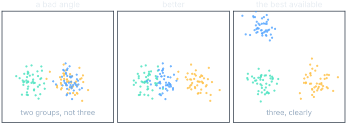
The three panels above are one cloud of points, photographed from three directions. Nothing about the data differs between them — those are genuine projections of the same list of points onto three different planes. Turn the flashlight and groups that were piled on top of one another come apart, or the reverse. A shadow always loses something, and which something it loses is a choice somebody made.

That is the whole tension of this chapter. The question is not "is this plot true" but "which of the true things did it choose to keep?"

Choosing the angle on purpose

If the angle is a choice, we should make it deliberately. The standard way of making it is PCA — principal component analysis — and stripped of its machinery it is one sentence: point the flashlight so the shadow is as spread out as possible.

The reasoning is that a direction along which the data barely varies carries almost nothing to distinguish one point from another, so losing it costs little. A direction along which the data varies a lot is doing real work, and we should keep it. So: rank every possible direction by how much the data spreads along it, and keep the top two.

Two housekeeping steps come first, and both matter. Center the data — subtract the average point — so that the readings describe displacement from the middle of the cloud instead of from an arbitrary origin. And use unit ruler directions, so a reading is a coordinate and not a coordinate multiplied by some leftover scale factor.

Now the second component. It must be at right angles to the first, which in two dimensions leaves exactly one choice: $[-0.8, 0.6]$. Its readings are 0, 0, 1, −1, so its variance is $2 \div 4 = 0.5$.

Add the two up: $12.5 + 0.5 = 13.0$. Now add up the two we started with: $4.82 + 8.18 = 13.0$. The same total. Turning the rulers moved the spread around between them but never created or destroyed any, and that conservation is what makes the next number meaningful.

In words: the first direction alone accounts for about 96% of all the spread in this cloud. Keep it and throw the other away, and you have lost 4% of what distinguished these four points.

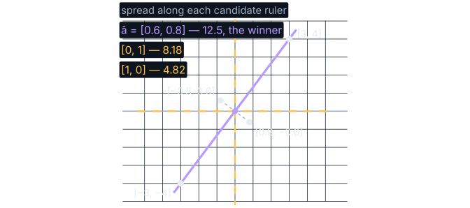
That percentage — the variance explained — is the single most important number on any embedding plot, and it is also the one most often left off. A two-dimensional shadow of a 1000-dimensional space frequently keeps less than 15% of the spread. The picture may still be worth looking at. But you are looking at a seventh of the evidence, and nobody has told you which seventh.

What a shadow is allowed to prove

Here is the part worth memorizing, because it turns "be careful with these plots" into two precise rules that point in opposite directions.

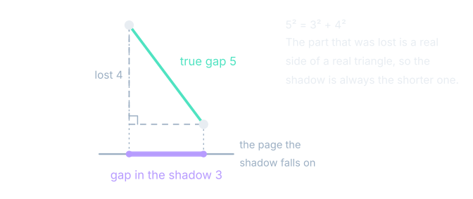
When a point is projected, its journey splits into two perpendicular pieces: the part that landed on the page, and the part that was lost. Those two pieces and the original form a right triangle, so Pythagoras applies to them — which gives us a hard guarantee.

In words: the original length squared equals the shadow's length squared plus the lost part's length squared. Because the lost piece can never be negative, the shadow is never longer than the original.

Apply that to the gap between two points and the two rules fall out:

• Distance in the shadow is never more than the true distance. So if two dots look far apart on the page, they really are far apart in the full space. A shadow cannot manufacture a separation that was not there.
• Distance in the shadow can be much less than the true distance. So two dots sitting on top of each other prove nothing whatever. They may be neighbors, or they may be on opposite sides of the space with their difference pointing entirely in a direction the projection discarded.

See it move

Turn the flashlight yourself. The cloud below has three real groups in three dimensions. Rotate the viewing direction and watch the groups merge and separate in the shadow beneath, with the share of spread kept reported live.

Where this shows up

• Every embedding visualization you will ever be shown. The first two questions are now automatic: what share of the spread does this keep, and is this a projection or a neighbor-preserving rearrangement? If the caption answers neither, the picture is decoration.
• Dimensionality reduction as a preprocessing step. Cutting 1000 dimensions to 100 before clustering or search is the same operation with more rulers kept. The AI/ML book's classical toolbox shows where it sits in a working pipeline.
• Reading a model's internals. When researchers look for structure inside a network's activations, they are projecting onto a handful of chosen directions and reading the shadow. The guarantees in this chapter are exactly the guarantees on their conclusions.
• Compression and storage. Keeping the top directions and discarding the rest is how a vector store shrinks its index, and the variance-explained figure is the honest statement of what that saving cost.

Where we're headed

That completes Part I. You now have the whole instrument kit — a space, two rulers, an honest account of what many dimensions do to both, and a way of looking at the result without fooling yourself. Every one of those was built without a single mention of machine learning, which was deliberate: none of them are machine-learning ideas. They are facts about space that machine learning happens to depend on.

The rest of this book puts meaning into that space — how positions get earned from the company a word keeps, how context moves a point, how a probability surface is read as surprise, and what the instruments at the frontier are actually measuring. Those parts are being written; the book's front page lists what is coming. In the meantime, the next rung of the ladder is AI/ML from the Ground Up, which takes the space you have just built and starts fitting things in it.