The map you built has a hole in it
A word does not have one position inside a language model. It has a starting position, and the first layer moves it somewhere else depending on what else is in the sentence.
The ten thousand Wikipedia points from the previous chapter were real, and the neighbor lists were real. Ask one question about them that the plot cannot answer: which sentence was each point in? For an article embedding that question is a category error, because the whole article went in. For a single word it is the only question that matters. "Bank" near a river and "bank" near a mortgage are the same four letters and the same row of a lookup table. If that row is all a model has, it cannot tell the two apart.
It isn't all a model has. This chapter runs one attention head on a two-word sentence, by hand, and watches the word the finish in two different places depending on the word in front of it. Everything you learned in Part II still holds, with one word changed: a counted position is where a word starts.
One token, two sentences
The toy is two dimensions wide, because two dimensions can be drawn and checked. I call axis 1 drink-ish and axis 2 animal-ish. The model has no such names. The names are mine, chosen so the arithmetic below means something while you read it, and nothing in the model ever consults them.
Three words, three starting positions:
drink at $[4.000,\ 0.000]$, length 4.000. feed at $[0.000,\ 4.000]$, length 4.000. the at $[1.000,\ 1.000]$, length 1.414.
Chapter 2's cosine says what those positions are to each other. Between drink and feed it is 0.000, so they are at right angles and share no direction at all. Between the and drink it is 0.707, because the sits on the diagonal and leans equally toward both.
Now two sentences, built to be mirror images of each other so the only difference between them is the first word:
S1 is the two words drink the, and S2 is the two words feed the.
Both end in the same token. That token enters the layer at $[1.000,\ 1.000]$ in both sentences, from the same row of the same table. The claim of this chapter is that it does not leave at $[1.000,\ 1.000]$, and that it does not leave at the same place in the two sentences.
A head asks every earlier position one question
An attention head at position 2 asks every position up to and including itself the same question: how much do you agree with me? The number it gets back is Chapter 1's dot product.
Think of a ship taking a bearing on the ship ahead. The heading you end up steering is your own heading blended with the one you are following, weighted by how much you trust the sighting. An attention head does the same blend with scores and weights.
Real heads do not compare the raw positions. They multiply each position by a learned matrix first. One makes the question being asked, called the query. One makes the thing being asked, called the key. One makes what a position hands over if it is picked, called the value. Those three matrices, and why a layer runs several heads at once, are taught in Attention in the LLM book.
In this toy all three matrices are the $2 \times 2$ identity. The head below is the simplest head that can exist, so its score is the dot product of two positions with nothing learned in between. What follows is about the steps after the scores, and those are the steps that survive when the matrices are real.
Worked example: two scores
The query is the position of the: $\mathbf{q} = [1.000,\ 1.000]$.
The keys are the positions of everything up to here. In S1 that is drink at $[4.000,\ 0.000]$ and the itself at $[1.000,\ 1.000]$.
Score against drink: $1.000 \times 4.000 + 1.000 \times 0.000 = 4.000$.
Score against itself: $1.000 \times 1.000 + 1.000 \times 1.000 = 2.000$.
The division that comes next is part of the definition, so write the whole thing down at once:
$$s_j = \frac{\mathbf{q} \cdot \mathbf{k}_j}{\sqrt{d_k}}$$In words: the score of earlier position $j$ is the dot product of my query with that position's key, divided by the square root of the number of dimensions. Here $d_k = 2$, so the divisor is 1.414, and the two scores 4.000 and 2.000 become 2.828 and 1.414.
The divisor is a thermostat. Dot products grow with the number of dimensions, and large scores make the next step lopsided, so the definition divides them back down. In a real model the key dimension is far larger than 2 and the divisor grows with it. Here it is 1.414, which is small enough that you can see what it does and large enough that it does something.
S2 gives the same two numbers. Its first word is feed at $[0.000,\ 4.000]$, and the dot product with $[1.000,\ 1.000]$ is $1.000 \times 0.000 + 1.000 \times 4.000 = 4.000$ again. The two sentences are mirror images, so they score identically, and every difference between the two answers comes from the mixture and not from the weights.
Scores become shares
Two scores, 2.828 and 1.414, are not yet an answer. They are not comparable to anything, they do not add to anything, and one of them could be negative. Softmax fixes all three at once:
$$a_j = \mathrm{softmax}(s)_j = \frac{e^{s_j}}{\sum_i e^{s_i}}$$In words: raise $e$ to each score, then divide each of those by their total. Exponentiating makes every number positive, and dividing by the total makes them add to one.
$$\sum_j a_j = 1$$In words: the weights add to one.
On our two scores that gives 0.804 and 0.196. Each one is an attention weight: the share of the output that this earlier position gets. Drink takes 0.804 of the output and the keeps 0.196 of itself.
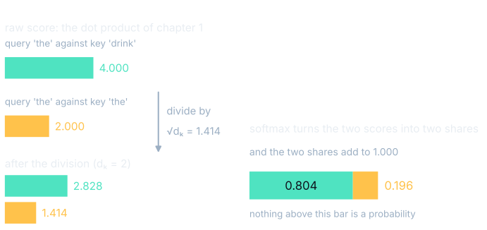
Softmax has two properties that matter here. It never returns a zero, so every earlier position gets some share, however small. And it reads the gaps between scores rather than their sizes, which is why the thermostat matters. Shrink every score toward zero and the shares even out. Blow them up and one share takes almost everything.
A weighted average is a point on a line
The head's output is the weighted average of what each earlier position hands over:
$$\mathbf{o} = \sum_j a_j \mathbf{v}_j$$In words: multiply each earlier position's value by its share, and add the results. With the value matrix set to the identity, position $j$'s value is its own position.
Worked example: the head output for S1
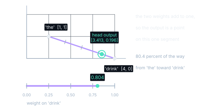
Across: $0.804 \times 4.000 + 0.196 \times 1.000 = 3.413$.
Up: $0.804 \times 0.000 + 0.196 \times 1.000 = 0.196$.
The output is $[3.413,\ 0.196]$, of length 3.419.
In words: the head's answer for the word the in the sentence drink the is a position most of the way over toward drink, with a little of the original left in it.
Because the two weights add to 1.000, that output cannot land just anywhere. It lands on the straight segment joining $[1.000,\ 1.000]$ and $[4.000,\ 0.000]$, at 80.4 percent of the way from the toward drink. Every output this head can produce, for any pair of weights, is a point on that one segment. The weights choose where on it.
The picture assumes the value matrix is the identity. Set the value matrix to $\begin{bmatrix}0 & 1\\ 1 & 0\end{bmatrix}$, which swaps a position's two coordinates, and change nothing else. The query and the keys are untouched, so the scores are still 4.000 and 2.000 and the weights are still 0.804 and 0.196. But drink now hands over $[0.000,\ 4.000]$ instead of $[4.000,\ 0.000]$, and the output is $[0.196,\ 3.413]$: the opposite corner of the plane.
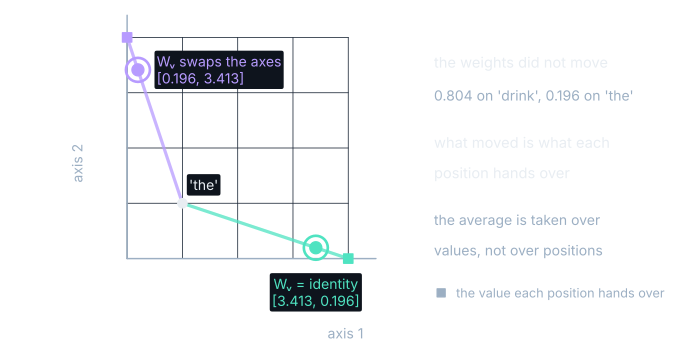
The head's output is a weighted average of what each position offers, and the segment picture holds only while the value matrix is the identity. In a real head the values are learned, and there is a fourth matrix after the average that maps the result again before it is written back. The output is still an average, but of the learned values, not of the positions you can see.
Two contexts, cosine 0.114
Run S2 the same way. The weights are the same 0.804 and 0.196, and feed hands over $[0.000,\ 4.000]$, so the output is $[0.196,\ 3.413]$ with length 3.419. The mirror image of S1, as designed.
Now put the before and after side by side. Before the layer, the was one position in both sentences, so its cosine with itself was 1.000. After the head it is two positions, $[3.413,\ 0.196]$ and $[0.196,\ 3.413]$, and the cosine between them is 0.114. That is an angle of 83.441 degrees. One token, two sentences, nearly perpendicular.
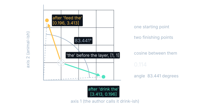
Nothing about the token changed. The embedding table was not consulted twice, the weights came out identical in both sentences, and no parameter moved. The only difference between the two runs is which word sat in front, and that was enough to send the same token to two places 83.441 degrees apart.
This is what people mean by a contextual embedding: the position of a token at some depth in a running model, which depends on the sentence it is in. It is a different object from the embedding-table row that Part II earned by counting, and the two get called by the same name constantly.
And it is added, not substituted
The head's output is not what the token becomes. It is what gets added to what the token already was. One plus sign:
Worked example: putting the original back
S1: $[1.000,\ 1.000] + [3.413,\ 0.196] = [4.413,\ 1.196]$, length 4.572.
S2: $[1.000,\ 1.000] + [0.196,\ 3.413] = [1.196,\ 4.413]$, length 4.572.
Cosine between those two: 0.505.
In words: adding the starting position back to both answers pulls the two versions of the toward each other, from a cosine of 0.114 to a cosine of 0.505.
The head output alone gives a cosine of 0.114; the position the rest of the stack sees gives 0.505. The head's output is a message, and the position that the rest of the stack sees is the token's old position with that message added on top. Something the token brought with it survives every layer.
| Step | S1 drink the | S2 feed the |
|---|---|---|
| Raw scores, query against the two keys | 4.000, 2.000 | 4.000, 2.000 |
| Divided by $\sqrt{d_k} = 1.414$ | 2.828, 1.414 | 2.828, 1.414 |
| Softmax weights | 0.804, 0.196 | 0.804, 0.196 |
| Head output $\mathbf{o}$ | [3.413, 0.196] | [0.196, 3.413] |
| Length of $\mathbf{o}$ | 3.419 | 3.419 |
| Cosine between the two head outputs | 0.114 | |
| Position after adding the original back | [4.413, 1.196] | [1.196, 4.413] |
| Cosine between the two positions | 0.505 | |
Read the first three rows across and they are identical, which is the mirror symmetry doing its job. Read row four and the two sentences part company. Only a table shows both facts at once.
Try it yourself
Both sentences below run live. Drag the context word anywhere in the plane and every number recomputes: the two scores, the two shares, both outputs, and the cosine between them.
One more thing to notice while dragging. Move the context word onto the itself and both scores become the same number, so the shares are half and half and the output sits at the midpoint. Move it to the origin and it scores zero against the query, which is what a right angle looks like in this arithmetic. Neither is a special case; the same arithmetic produces both.
Where you'll meet this
- The word "embedding" on a product page. An embedding API that takes a sentence and returns one vector is doing something different from an embedding table that takes a token and returns its row. The first ran a model and pooled the contextual positions; the second did a lookup. Both get called embeddings, and the difference is this chapter.
- Retrieval indexes. A vector index built from word vectors stores the starting positions, so every sense of a word shares one entry. An index built from a model's contextual output stores positions that depend on the surrounding text, so the same word in two documents lands in two places. Neither is wrong; they answer different questions, and mixing vectors from the two in one index gives you a space with no shared meaning at all.
- Mechanism you already have. The query, key and value matrices, the reason a layer runs several heads at once, and what a real attention pattern looks like over a real sentence are all in Attention in the LLM book. This chapter took that mechanism as given and asked one question about it: where does the point end up?
What you now know
- A token's position inside a model is not a property of the token. The embedding-table row is where it starts, and every layer moves it.
- An attention head scores each earlier position with Chapter 1's dot product, divides by the square root of the key dimension, and turns the scores into shares that add to 1.000.
- Because the shares add to one, the head's output is a point on the segment joining the values it averaged, 80.4 percent of the way from the toward drink in our sentence.
- That segment is drawn between values rather than between token positions, and swapping the value matrix moves the output to the opposite corner of the plane without changing a single weight.
- The same token the leaves the head at two positions whose cosine is 0.114 in the two mirror sentences, and at two positions whose cosine is 0.505 once the original is added back, which is the number the rest of the stack works with.
- The thing you now know exists is the contextual embedding, and that the phrase "the vector for a word" meant a table row before 2018 and a position inside a running model after it.
Where we're headed
We added the head's output back to the position it came from and got $[4.413,\ 1.196]$. That plus sign is not a detail of this layer. It is how the whole stack is wired: one running position per token, and every block reading it and adding to it, twenty-four or ninety-six times over. The next chapter follows one position all the way through, adds up thirteen rows of a table to check that the finish is the start plus every write, and finds a layer that undoes part of what an earlier layer did.