Nobody drew the map
A word's coordinates come out of a procedure run over text, with no human judgment about meaning inside it. This chapter is that procedure.
The last chapter taught us to distrust a picture: a few hundred colored dots on a pair of axes, with clusters labeled "sports," "medicine," "recipes." I never asked who put the dots there. I don't think most people do. Somebody made that plot from a list of coordinates, and nobody typed them. No lexicographer decided that tea belongs at 6 across and 0 up. By the end of this chapter you will have built such a list by hand, out of ten dull sentences and a stack of tally marks. You will also be able to say what its coordinates mean and where they lie to you.
Know a word by the company it keeps
The idea underneath every embedding ever trained is older than computers. The linguist Zellig Harris wrote it down in 1954, and John Firth gave it the sentence everybody quotes in 1957: “You shall know a word by the company it keeps!”
The distributional hypothesis says that words which turn up in the same surroundings tend to mean similar things, because using a word the same way is most of what meaning the same thing amounts to. Hand someone a sentence with a word blanked out, "she poured herself a cup of ______ and let it cool," and they can rank the candidates without a dictionary.
This is a claim about text, and claims about text can be wrong. It would be false if words with similar meanings routinely appeared in different company, and it is partly false in the place you would expect. Hot and cold keep almost identical company, and they are opposites. That bites us before the chapter is over.
What makes the hypothesis useful is that "the company it keeps" is countable. A claim about meaning becomes arithmetic a clerk could do.
Counting the company
Our entire corpus is ten sentences, deliberately dull, about six things and what people do with them.
The corpus
- Drink your tea, drink your coffee.
- Hot tea, hot coffee, hot milk.
- We drink coffee and drink milk.
- Hot tea and milk to drink.
- Drink the tea while it is hot.
- Feed the cat milk, feed the dog.
- We walk the dog, then walk the dog again, and walk the cat.
- We walk the horse, feed the horse, and walk the horse again.
- Feed the dog and feed the cat.
- Give the cat a drink, give the dog a drink, give the horse a drink.
Six words interest us, tea, coffee, milk, dog, cat, horse, and we will describe each by how often four other words show up near it: drink, hot, feed, walk. Those four are the questions we are asking, and choosing them is the one human decision in the procedure.
"Near" needs a definition, and this is it: a context window of two words either side. Walk the corpus one word at a time. Every time you land on one of our six, look two words left and two words right, and put a tally mark against every one of the four context words you see. Never look past the end of a sentence.
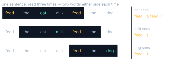
Do that for all ten sentences and you get this. Every number was counted, not chosen.
| word | drink | hot | feed | walk |
|---|---|---|---|---|
| tea | 3 | 3 | 0 | 0 |
| coffee | 3 | 2 | 0 | 0 |
| milk | 2 | 1 | 1 | 0 |
| dog | 1 | 0 | 3 | 3 |
| cat | 1 | 0 | 3 | 1 |
| horse | 1 | 0 | 2 | 3 |
That grid is a co-occurrence matrix. Milk is the interesting row, because milk is drunk by people and fed to the cat, and its row says so with a 2, a 1 and a 1.
The counts are the coordinates
Each row of that table is a list of four numbers, and Chapter 1 told us a list of numbers is a position. So each row is a position, in a space with one axis per context word. The step is small enough to miss.
$$\mathbf{v}_{\text{tea}} = [3,\ 3,\ 0,\ 0], \qquad \mathbf{v}_{\text{cat}} = [1,\ 0,\ 3,\ 1]$$In words: the vector for tea reaches 3 along the drink axis, 3 along the hot axis, and nothing at all along feed or walk. The vector for cat reaches 1 along drink, nothing along hot, 3 along feed and 1 along walk. Each word's four tallies are its four coordinates, in that order, and there is nothing else in there.
A word represented as a list of numbers like this is called an embedding: numbers standing in for a thing, positioned so that measuring them tells you something. Ours were counted by hand. A real one is trained, which Chapter 7 covers, and a trained one is the same kind of object, in the same kind of space, measured with the same two rulers from Chapter 2.
Two numbers you can plot
Four dimensions will not go on a page, and Chapter 4 told us what to do about that: choose a couple of directions and take readings along them. Two choices here need no machinery. Add the two drink-ish columns for the across reading, and the two animal-ish columns for the up reading.
$$x = c_{\text{drink}} + c_{\text{hot}}, \qquad y = c_{\text{feed}} + c_{\text{walk}}$$In words: a word's horizontal position is how often it was seen near drink plus how often it was seen near hot. Its vertical position is how often it was seen near feed plus how often it was seen near walk. Two additions per word, and the map is finished.
| word | x = drink + hot | y = feed + walk | length |
|---|---|---|---|
| tea | 6 | 0 | 6.000 |
| coffee | 5 | 0 | 5.000 |
| milk | 3 | 1 | 3.162 |
| dog | 1 | 6 | 6.083 |
| cat | 1 | 4 | 4.123 |
| horse | 1 | 5 | 5.099 |
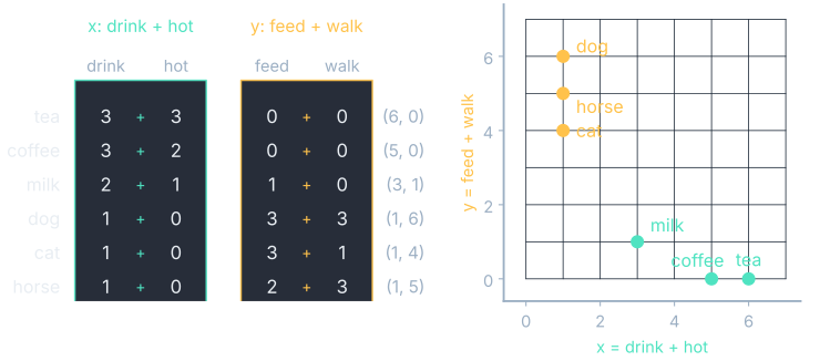
Nobody told this map that tea and coffee are similar, or that a dog is not a beverage. The grouping is a consequence of the tallies, and the tallies are a consequence of the sentences.
If you suspect I picked those two sums to flatter the result, run Chapter 4's method on the counts instead of guessing. Principal component analysis, given the centered count table and no hints, puts 87.7% of the spread on a single direction whose weights are −0.400 on drink, −0.500 on hot, +0.544 on feed and +0.543 on walk. That is drink-and-hot pulling against feed-and-walk: the axis I chose by eye, discovered from the data by a procedure that never saw my choice.
One piece of bookkeeping before we measure anything, because Chapter 4's guarantee depends on it. These two sums are a projection scaled up by the square root of two. Divide both coordinates by 1.414 and Chapter 4's shrink guarantee holds, as you can check.
What the flattening cost
Chapter 2 gave us the ruler for this: the cosine of the angle between two vectors, which ignores length and scores only heading.
$$\cos\theta = \frac{\mathbf{v} \cdot \mathbf{u}}{\|\mathbf{v}\|\,\|\mathbf{u}\|}$$In words: multiply the matching coordinates of the two vectors and add up the products, then divide by both of their lengths. One means the same heading, and zero means at right angles.
Tea and coffee, scored twice
On the four counts. The dot product is $3 \times 3 + 3 \times 2 + 0 + 0 = 15$. The lengths are $\sqrt{9 + 9} = 4.243$ and $\sqrt{9 + 4} = 3.606$. So the cosine is $15 \div (4.243 \times 3.606) = 15 \div 15.297 = 0.981$: very close, and not identical, because tea shows up near hot three times and coffee only twice.
On the map. Tea is at $[6, 0]$ and coffee at $[5, 0]$. The dot product is 30, the lengths are 6 and 5, and $30 \div 30 = 1.000$.
In words: the one real difference between tea and coffee lived in the direction our two sums threw away, so on the map the two words share a heading to as many decimals as you care to print.
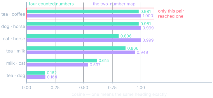
Every claim I am about to make about this map is a claim about a shadow. The separation between drinks and animals is real, because after that rescaling a shadow cannot manufacture distance. Cosine carries no such guarantee in either direction: the flattening pushed tea and coffee together and pushed milk and cat apart, and the figure above shows both.
Does it know anything?
Pick a word, score it against the other five with cosine, and sort. Starting from tea, on the four counts:
| word | cosine with tea |
|---|---|
| coffee | 0.981 |
| milk | 0.866 |
| cat | 0.213 |
| horse | 0.189 |
| dog | 0.162 |
There is a gap of more than six tenths between milk and cat. The drinks are a group, the animals are a group, and the procedure that found them counted words. It never learned what a drink is, or anything at all in the sense we normally mean.
Milk is the word worth staring at. Against the drinks it scores 0.866 and 0.906; against the animals, 0.436 to 0.615. It is neither, and its position summarizes the fact that we drink it and also pour it in the cat's bowl. The method is reporting accurately that the word is used both ways, and a single position is the price of saying so in one place on a map.
Try it yourself
The corpus below is editable and the window is a dial. Change either one and watch the tally grid and the map change together, because the positions are downstream of the counts and have no other source.
What the real ones do differently
- Raw counts are a poor measure of association. The is near everything, so real systems first divide out how common each word is on its own, a correction called pointwise mutual information.
- The matrix is enormous and mostly zeros. A vocabulary of 50,000 words against 50,000 contexts is 2.5 billion cells, nearly all empty, so it is factored down to a few hundred dense columns, which is Chapter 4's move again at scale.
- The good ones are trained, not just tallied. Word2vec (Mikolov and colleagues, 2013) learns positions by prediction rather than counting. GloVe (Pennington and colleagues, 2014) still counts, fitting its vectors directly to the logged co-occurrence tallies by weighted least squares, but it learns the fit rather than factoring the table outright. Either way the positions are trained, which is the subject of Chapter 7.
- Those two families are closer than they look. Levy and Goldberg's Neural Word Embedding as Implicit Matrix Factorization (2014) showed that word2vec's skip-gram objective is, under the hood, factoring a corrected count matrix. That is a result about one method rather than about every embedding, and it means the table you built by hand and a trained embedding are far closer than they look.
Where you'll meet this
- Every vector search and every recommendation. The ranking is a cosine between positions earned from company kept, which is why a search engine can match a passage sharing no words with your query, and why it sometimes matches wording rather than topic.
- The first layer of a language model. Its embedding table is one row per token, trained rather than counted; the Q&A answer on embeddings lays out how that lookup differs from a search embedding, and Meaning as Direction works the ready-made arrows.
- Every dataset audit you will ever run. If a corpus only discusses a group of people in one kind of sentence, those words take their positions from that company, and tuning downstream does not un-count it.
- Reading a model card. "Trained on web text with a context window of n" is the same two settings you just changed by hand: what the company is, and how near counts as near.
What you now know
- A word's coordinates are not assigned by anyone; they are a summary of the company it keeps, built by counting neighbors inside a window somebody chose.
- A row of a co-occurrence table is already an embedding: four tallies are four coordinates, and Chapter 2's rulers measure them without modification.
- Cosine ranking on our six words separates drinks from animals with a gap of more than six tenths, and it does so having counted words rather than understood them.
- Flattening four counts to two plottable numbers pushed tea and coffee from 0.981 to 1.000, so the picture claims an identity the data never contained.
- The field with a name for all of this is distributional semantics, and one of its central results is that a corrected count matrix and a trained embedding are far closer to the same object than they look.
Where we're headed
We have positions now, earned rather than asserted, and we can measure them. The next thing everyone does with an embedding space is arithmetic on it: subtract one position from another, add the difference somewhere else, and land on a word that was never mentioned. King minus man plus woman equals queen is the demonstration that made these spaces famous.
The next chapter does it twice. Once on a map built so that it works, where the whole thing closes into a parallelogram you can check by hand. Then on the map we just built from real counts, where the same procedure returns the wrong word, and where finding out why turns up a rule every implementation applies silently and almost no write-up mentions.