Everything so far, on real data
This chapter runs every operation from the last four on a corpus I did not write, and the results are messier in ways worth seeing.
Every number in the last four chapters came out of ten sentences I wrote myself. That was the point, because you could check all of it with a pencil. It also means that map could never tell me anything I had not put into it. So: ten thousand article introductions from Simple English Wikipedia, 1,250 from each of eight subjects, each turned into 384 numbers by a small open model running on my laptop with no cloud service involved. The text is CC BY-SA 4.0 and GFDL, the model is Apache-2.0, and one script fetched, embedded and packed it and prints every number below.
The operation has not changed since Chapter 5: look at the company a thing keeps, turn that into coordinates. A trained network does the looking instead of tally marks, and there are 384 coordinates instead of two.
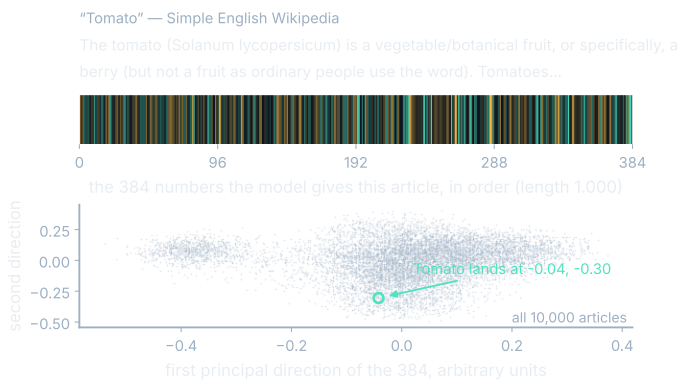
One question runs under the whole chapter. When you look at a picture of an embedding space and see tidy, well-separated clusters, how much of that space are you looking at?
| Field | Value |
|---|---|
| Source | Simple English Wikipedia article introductions |
| Retrieved | 2026-09-23, through the Wikimedia Action API |
| License (text) | CC BY-SA 4.0 and GFDL — attribution and share-alike |
| Articles | 10,000, exactly 1,250 in each of 8 subjects |
| Text embedded per article | the first 400 characters of the introduction |
| Model | sentence-transformers/all-MiniLM-L6-v2 |
| License (model) | Apache-2.0 |
| Dimensions | 384 |
| What you download | 1.92 MB of titles and 7.68 MB of numbers — 9.6 MB in total, and only when you press the button |
First safari
Pick something you know and ask the map what is near it. The score is Chapter 2's cosine, unchanged except for how many terms it has:
$$\cos(\mathbf{v},\, \mathbf{u}) = \frac{\mathbf{v} \cdot \mathbf{u}}{\|\mathbf{v}\|\,\|\mathbf{u}\|} = \frac{\sum_{i=1}^{384} v_i u_i}{\|\mathbf{v}\|\,\|\mathbf{u}\|}$$In words: multiply the two articles' first numbers, then their second numbers, and so on for all 384; add up the 384 products; divide by both lengths. It is the arithmetic we did by hand with two numbers, done 384 times. Every article here was scaled to length one, so both divisions are by one and the sum is the whole story.
I asked for Tomato. Its nearest is Tomatillo at 0.531, and the list is fruit and vegetable articles all the way down, apart from eighth place, which is Fruit Ninja, a mobile game about slicing fruit, at 0.427. It is near because its opening paragraph is worded like the others, not because it shares a subject, and wording is the only evidence the model ever had.
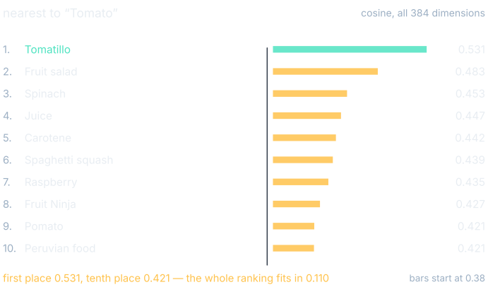
Compare that to the six-word map, where cocoa scored 0.997 against milk and under 0.5 against every animal. Here the whole top ten fits inside 0.110, every answer is plausible, and the order turns on differences you would not see at two decimals.
What Chapter 3 actually promised
This is the first space in the book with enough dimensions for Chapter 3's warning to apply, so it is the place to say what that warning said. It was proved for Euclidean distance between points drawn at random: as dimensions pile up, the furthest point in a random set stops being meaningfully further than the nearest, and the ratio between those distances collapses toward one.
Both halves matter, and the second is the one that rescues us. In 384 dimensions two directions chosen at random sit at almost a right angle, missing by an amount the dimension count fixes:
$$\text{spread of cosines between random directions} \approx \frac{1}{\sqrt{d}} = \frac{1}{\sqrt{384}} = 0.051$$In words: pick two directions at random in 384 dimensions and their cosine will land near zero, typically within about 0.051 of it. The measured spread for 384 random directions in this corpus's own arithmetic is 0.051, which is the prediction arriving to three decimal places.
Real articles do not behave that way. Their pairwise cosines average 0.033 with a spread of 0.088, nearly twice as wide as random, because these points are the output of a model trained to put related wording in related places. Run Chapter 3's own quantity on its own metric: across a thousand neighbors the furthest-over-nearest distance ratio is 1.459 for real articles and 1.077 for random directions. Concentration is hitting the random set hard and ours barely at all.
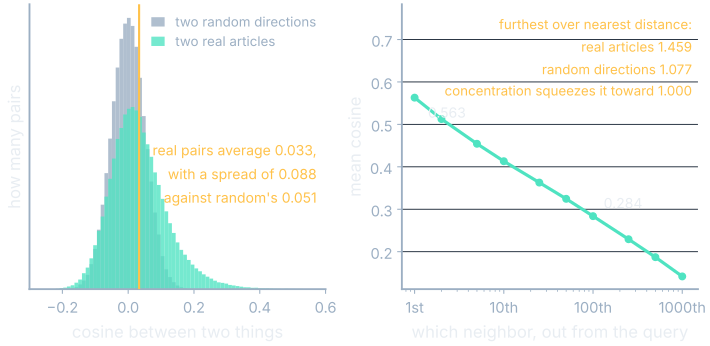
What does bite is the right-hand curve. The average nearest neighbor scores 0.563, the tenth 0.413 and the hundredth 0.284, so your top ten is barely separated from your top hundred, and every index that skips part of the set, which is all of them, is trading in a currency this narrow.
Reading the shadow
Now the picture everybody publishes. Flatten all 384 numbers onto the two directions holding the most spread, which is Chapter 4's method run on real data, and plot it.
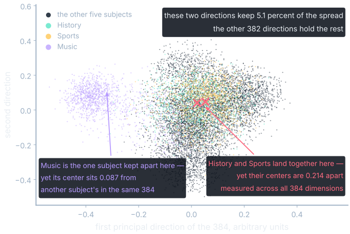
Two directions out of 384 keep 5.1 percent of the spread. The other 382 hold everything else that distinguishes these articles, and that remainder is the evidence that did not fit on a screen rather than noise.
Chapter 4's rule is asymmetric, and here the asymmetry earns its keep. A shadow can only bring things closer together, never push them apart, so two dots far apart on that plot are far apart in all 384 dimensions, while two dots close together tell you nothing. Name the metric before leaning on the guarantee: it holds for straight-line distance between the centered vectors, which is what the projection preserves, and it is not a promise about cosine.
The figure carries the proof of both directions at once. History and Sports sit on top of each other, and their centers are 0.214 apart in the full space. Music looks like the one clean, separate subject in the picture, and its center sits 0.087 from another subject's, which is closer than the pair the picture merged. The separation you can see is the least trustworthy thing on the page.
Cluster spelunking
The clusters tab runs Chapter 8's k-means on the real 384-dimensional vectors rather than on the flattened picture, because grouping on a shadow would group things that were never together.
Ask for three groups and you get three, and you will name them in seconds: food and science, places and teams and vehicles, music. Ask for nine and the music group of 1,505 comes apart into 377 articles about bands and 902 about songs. That split is not rock against pop. It is articles about groups of people against articles about recordings, a fact about how introductions are written rather than about music.
Nothing in the method found three groups or nine. It produced the number I asked for, both times, and named none of them. The names are mine, and in a slide deck they look like findings.
Centroid games
The centroids tab averages every article in one subject, which is Chapter 8's operation on 384 coordinates instead of two:
$$\mathbf{c} = \frac{1}{k}\sum_{i=1}^{k} \mathbf{v}_i$$In words: add up the positions of all the articles in the subject, coordinate by coordinate, and divide each total by how many there were. The result is one position standing in for the whole subject, scaled back to length one afterward so it can be compared by cosine like everything else.
Take History. Its 1,250 members sit an average of 0.274 from their own centroid, which is low. The five articles nearest that centroid are all accounts of massacres and coups, so this is a centroid of atrocity reporting rather than of "history," which is what most of the subject's wording turned out to be. One of the five is filed under Food and drink: it is the Holodomor, and a famine sits in a food category.
Then look the other way. The History article furthest from the History centroid is General American English, at −0.034, a member pointing slightly away from its own set's average and further off than two articles picked at random. The arithmetic never complained. A centroid claims a set has a middle, and a Wikipedia subject usually does not have one.
Where it is wrong
I went looking for the opposite failure: two articles that ought to be neighbors and are not. The pair I found is Teddy Grahams and Golden Grahams, two supermarket products, both filed under Food and drink, both named after the same cracker. Their cosine is −0.009, and Golden Grahams sits 6,431st on Teddy Grahams' list of ten thousand.
So I went to look at why, which is the whole reason to walk your own data, and the answer was not in the geometry. The text stored for Teddy Grahams in this corpus is the opening of an article about a Japanese cartoon. Simple English Wikipedia's Teddy Grahams page was vandalized on 19 September 2026, four days before I fetched it, and the fetch took what was there. The model then did its job: it placed that paragraph next to Sonic Drive-In at 0.444, which is where a paragraph about Sonic belongs.
Nothing in the pipeline could have caught that. The embedding was right about the text, the text was wrong about the world, and every downstream number inherited the error silently. I am shipping it rather than swapping in a clean article, because the most useful thing a real corpus teaches is that most of what looks like a model failure is a data failure wearing a model's coat.
Make your own tonight
Everything on this page came off a laptop in an evening, and the recipe is four lines long. Get some text you care about: your own notes, a folder of reports, a series of meeting minutes. Cut it into pieces of a few hundred characters. Run each piece through an embedding model you downloaded; the one used here is about ninety megabytes, Apache-2.0, and embeds ten thousand pieces in under a minute on a plain CPU. Keep the numbers in a file beside the text.
At ten thousand pieces you need no index, no database and no service: a full scan is a few million multiply-adds, as Chapter 8's arithmetic predicted.
Within an hour of walking your own data you will find a neighbor you cannot explain. Chase it down. That one neighbor will teach you more about embeddings than the rest of this book, because it is the only part nobody can write for you.
See it move
Where you'll meet this
What you now know
- A real embedding space is the six-word map's operation at scale: ten thousand Wikipedia introductions, 384 numbers each, built by one script from licensed text and an Apache-2.0 model on a laptop.
- Real neighbor lists are tight and strange: Tomato's ten nearest all fall inside 0.110 of each other, and the eighth is a mobile game about slicing fruit.
- Chapter 3's concentration result was proved for Euclidean distance between random points, and this corpus is not random: its furthest-over-nearest ratio is 1.459 where random directions give 1.077.
- The best two-dimensional picture of this corpus keeps 5.1 percent of the spread, so it can prove two things are far apart and can never prove they are close.
- Clusters arrive unnamed and in whatever quantity you asked for, and asking for more often splits on how articles are written rather than on what they are about.
- Most of what looks like a model failure is a data failure: two products that should be neighbors sit 6,431 places apart because one article had been vandalized four days before I fetched it, and embedding drift between model versions leaves two spaces with no shared axes at all.
Where we're headed
That closes the second act. We started with a space that had no meaning in it, put meaning in by counting, argued about what arithmetic on positions proves, learned to search the result, and have now walked a real one with the warnings printed on the same plot. The remaining question is where these positions come from inside an actual language model. They are the first layer of a much larger machine, one that spends its whole time moving positions around, rather than a separate lookup table. Chapter 10 starts with the fact that breaks the map: run the same word through a model twice, in two different sentences, and it does not come out in the same place. That is the next act.