One point per document
A vector database gives every document one point, and that point has a capacity. This chapter measures it.
Since Chapter 8 you have been storing documents as positions and answering questions by looking near a query. Chapter 9 did it with ten thousand real Wikipedia paragraphs. Neither chapter asked the obvious follow-up question. A document is a few hundred words with dates and names and one serial number in it, and we are compressing all of that down to 384 numbers, or 768, or 1,536. What fits, and what gets left behind?
The answer is sharper than "it depends on the model," and most of it comes out of a three-by-three grid of numbers. The same grid says what a retrieval system's dimension buys, why serious search stacks have a second stage, and what that stage costs in milliseconds.
Two shapes of scorer
Everything that scores a query against a document has one of two shapes, and they differ over when the document is read.
A bi-encoder encodes the document on its own, stores the resulting vector, and later encodes the query on its own. The score is the dot product of the two. That is what chapters 8 and 9 were doing, and what a vector database is built around.
A cross-encoder takes the query and the document together, as one input, and returns a number. There is no document vector and no query vector. There is one model, reading a pair.
The Navy version of this: a silhouette card is drawn in advance and can be held against a thousand contacts an hour. A boarding party answers questions the card never anticipated, and you can send one out a few times a day. That is the trade.
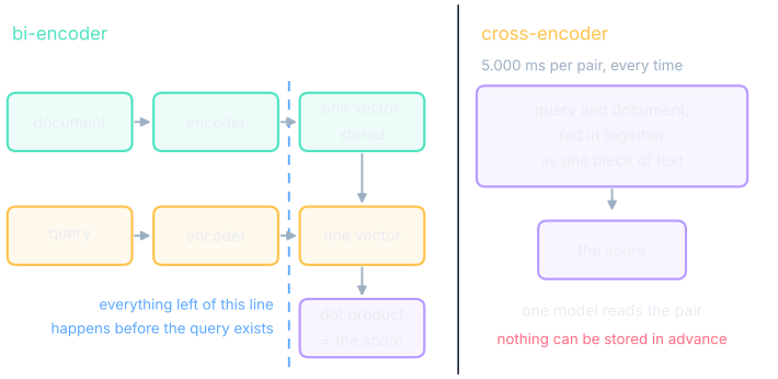
Because the bi-encoder's document arm runs early, it has to commit. Whatever it records about a document, it records before knowing what anybody will ask. The cross-encoder decides afterward.
The score matrix is a product
Write down every score a bi-encoder produces on a fixed set of queries and documents, and you get a grid: one row per query, one column per document. Call it $S$. Because each score is a dot product of a query vector with a document vector, that grid is a product of two thin matrices.
$$S = \mathbf{Q}\mathbf{D}^\top \quad \Rightarrow \quad \mathrm{rank}(S) \le d$$In words: stack the query vectors into $\mathbf{Q}$ and the document vectors into $\mathbf{D}$, both of them $d$ columns wide, and the whole score grid is one multiplied by the other's transpose. A product of two $d$-column matrices has rank at most $d$. The dimension is a ceiling on how many independent things the scores can say: no matter how many queries and documents you have, the grid can only carry $d$ worth of independent structure.
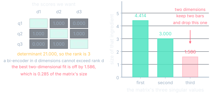
That makes a testable claim. Pick a grid of scores and ask whether a bi-encoder of a given size can reproduce it to the last decimal. Three queries, three documents, and these targets:
| d₁ | d₂ | d₃ | |
|---|---|---|---|
| q₁ | 3.000 | 1.000 | 0.000 |
| q₂ | 1.000 | 3.000 | 1.000 |
| q₃ | 0.000 | 1.000 | 3.000 |
Worked example: the determinant, by hand
Expand along the top row. Each entry is multiplied by the determinant of the two-by-two block left when you delete its row and column, with alternating signs:
$$\det S = 3(3\cdot 3 - 1\cdot 1) - 1(1\cdot 3 - 1\cdot 0) + 0 = 3 \times 8 - 3 = 21$$Read the result. The determinant is 21.000, which is not zero, so the three rows are independent and the rank is 3.
In words: no bi-encoder with fewer than three dimensions can produce this grid of scores, because a two-dimensional one can only reach grids of rank 2 or less, and this one has rank 3.
How far off would the best two-dimensional attempt be? Take the grid's three singular values, which are 4.414, 3.000 and 1.586. A rank-2 approximation keeps the first two and throws the third away, so the error is 1.586, which is 0.285 of the grid's size. The third ingredient is more than a quarter of the thing, so it is not a rounding artifact waiting to be squeezed out by a better training run.
That settles the question for exact scores. It does not settle the question anybody cares about.
Ranking is a weaker demand
Retrieval does not need the scores. It needs the order. Nobody checks whether q₁'s score on d₁ came out at 3.000; they check whether d₁ came back first. Asking for a specific grid of numbers is a much stronger request than asking for a specific ranking, and the rank bound answers the strong request only.
So test the weak one. Three queries and three documents again, with one demand: each query must rank its own document first. Draw 20,000 random pairs of two-dimensional arrangements and count how many satisfy it. The answer is 521 of 20,000. Two dimensions can order this case, and it happens by accident roughly one time in forty, even though the score grid we started from has rank 3.
A pattern two dimensions could not order
Orderings can still be out of reach. Showing it takes a harder demand than one rank calculation, and this one is small enough to hold in your head. Four documents. One query for every pair of them, so six queries. Each query has to put its own two documents above the other two. Nothing about the scores, only about which two come out on top.
Searching for an arrangement that satisfies all six at once, by random restart and hill-climbing on the worst query's margin, gives this:
| Dimensions | Best worst-case margin found | What that means |
|---|---|---|
| 2 | −0.000 | the search never got a query's own two documents strictly above the other two |
| 3 | 1.126 | all six queries answered, with room to spare |
| 4 | 1.116 | all six queries answered |
In words: the margin is the smallest gap, across all six queries, between the lower-scoring of a query's own two documents and the higher-scoring of the other two. A positive margin means every query is answered. The number crosses zero somewhere between two dimensions and three.
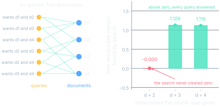
The −0.000 at two dimensions comes from a search: a hill climb that never got above zero. It shows that we could not find an arrangement that works, and it does not prove that none exists.
The theorem is somebody else's. Weller, Boratko, Naim and Lee's On the Theoretical Limitations of Embedding-Based Retrieval (2025) proves the general statement: the number of top-k subsets of documents that any query can pull out of a fixed set of embeddings is capped by the dimension. They then build a dataset, LIMIT, whose queries are trivial to state and whose required subsets exceed what current models' dimensions can express, and current models fail on it. That paper is the citation for the bound. Our six pair-queries are a small instance of the same shape, worked in the plane so you can see it.
One dimension per document always works
The cheapest way to see what dimension is buying is to stop compressing. Give each of the four documents its own axis, so d₁ is (1, 0, 0, 0), d₂ is (0, 1, 0, 0), and so on. Give the query that wants documents 1 and 2 the vector (1, 1, 0, 0). Its scores come out 1.000, 1.000, 0.000, 0.000, so its own two documents are on top with a margin of 1.000, and the same works for all six queries.
| Query | d₁ | d₂ | d₃ | d₄ | Top two |
|---|---|---|---|---|---|
| wants d₁ and d₂ | 1.000 | 1.000 | 0.000 | 0.000 | d₁, d₂ |
| wants d₁ and d₃ | 1.000 | 0.000 | 1.000 | 0.000 | d₁, d₃ |
| wants d₁ and d₄ | 1.000 | 0.000 | 0.000 | 1.000 | d₁, d₄ |
| wants d₂ and d₃ | 0.000 | 1.000 | 1.000 | 0.000 | d₂, d₃ |
| wants d₂ and d₄ | 0.000 | 1.000 | 0.000 | 1.000 | d₂, d₄ |
| wants d₃ and d₄ | 0.000 | 0.000 | 1.000 | 1.000 | d₃, d₄ |
Four documents, four dimensions, every query answered. That arrangement is useless in practice, because a corpus of a million documents would need a million dimensions and the index would be larger than the corpus. But it locates the cost. The difficulty was never in the geometry. It was in the compression, and the dimension is the compression ratio.
What the cross-encoder does instead
A cross-encoder's score is an arbitrary function of the pair. There is no grid factored into two thin matrices, so nothing in the last three sections applies to it.
Work one instance. The query is a serial number, RT-4419, and there are four passages. A cross-encoder that scores 1.000 when the passage contains that exact string and 0.000 when it does not gives:
| Passage | Text | Score |
|---|---|---|
| p₁ | replacement filter RT-4419, ships Tuesday | 1.000 |
| p₂ | replacement filter RT-4491, discontinued | 0.000 |
| p₃ | filters and cartridges, full catalog | 0.000 |
| p₄ | RT series filters: sizing guide | 0.000 |
Look at p₂. It differs from p₁ by two transposed digits, and in every way a topic model would measure, the two passages are the same passage. A bi-encoder has to decide whether RT-4419 and RT-4491 get different coordinates before either query is written, out of a fixed budget of dimensions, and it has to make that decision for every serial number in the catalog at once. The cross-encoder makes it after the query arrives, for one pair, and then forgets it.
The bi-encoder's problem is that it has to be ready for questions it has not heard.
The price of reading both
The cross-encoder's freedom costs time, and the arithmetic is one line.
$$T_{\text{rerank}} = t_q + t_{\text{ann}} + k\,t_{\text{pair}}$$In words: the time for one query is the time to embed it, plus the time for the approximate search over the stored vectors, plus the per-pair cost of the cross-encoder multiplied by how many documents you hand it. Only the last term grows with how much reranking you do.
Take 1,000,000 documents, 5.000 ms per cross-encoded pair, 8.000 ms to embed a query and 12.000 ms for the approximate search from Chapter 8.
| Approach | Arithmetic | Per query |
|---|---|---|
| cross-encode everything | 1,000,000 × 5.000 ms | 5,000.000 s = 83.333 min |
| retrieve 1,000, rerank 10 | 8.000 + 12.000 + 10 × 5.000 | 70.000 ms |
| retrieve 1,000, rerank 50 | 8.000 + 12.000 + 50 × 5.000 | 270.000 ms |
| retrieve 1,000, rerank 100 | 8.000 + 12.000 + 100 × 5.000 | 520.000 ms |
| retrieve 1,000, rerank 200 | 8.000 + 12.000 + 200 × 5.000 | 1,020.000 ms |
Rerank-50 is 18,518.519 times faster than cross-encoding the corpus. At an hour and twenty-three minutes per query, cross-encoding the whole corpus cannot serve anyone.
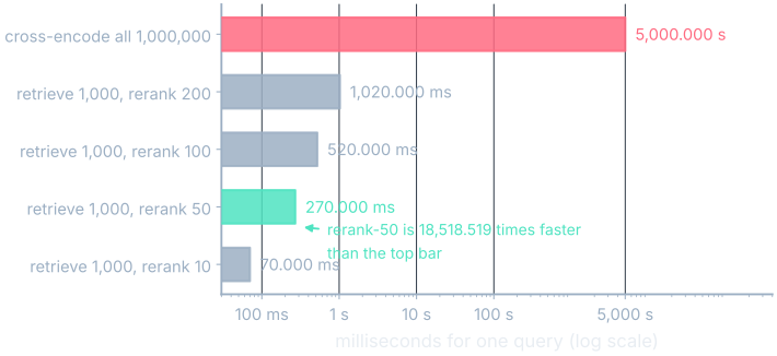
Notice also what the reranking term does not contain. The corpus size appears in the first row and nowhere else. Growing from a million documents to ten million changes the approximate-search cost only slowly (this model holds it fixed at 12.000 ms, which real indexes do not quite do) and leaves the rerank cost alone, because the rerank cost is set by $k$, the number of documents you chose to look at closely.
| Dimensions | Bytes per document | Per million, float32 | Per million, float16 |
|---|---|---|---|
| 384 | 1,536 | 1.536 GB | 0.768 GB |
| 768 | 3,072 | 3.072 GB | 1.536 GB |
| 1,536 | 6,144 | 6.144 GB | 3.072 GB |
So you do both
The standard arrangement puts the two scorers in series. Stage one is the bi-encoder with its stored vectors and its approximate index, and it returns a few hundred or a few thousand candidates fast. Stage two is the cross-encoder, which reads each surviving pair and re-sorts them.
One property of that arrangement is the failure mode nobody notices. Stage one's recall is a ceiling on stage two. A document that the bi-encoder did not return cannot be rescued by the reranker, which never sees it. If your stage-one recall at 1,000 is 0.900, then a perfect reranker gives you 0.900, and every hour spent improving the reranker is spent under that ceiling. When a two-stage system disappoints, measure stage one's recall first.
There is a middle option between the two shapes. Late-interaction models such as ColBERT store one vector per token rather than one per document, and score by matching a query's tokens against a document's tokens at query time. That buys back some of the capacity the single vector gave up, and it pays in storage, which is the same trade this chapter has been measuring from the other end. Khattab and Zaharia's ColBERT (2020) is the paper. For the plain two-stage form, Nogueira and Cho's Passage Re-ranking with BERT (2019) is the one that made it standard practice.
Run it yourself
The interactive opens on the six pair-queries with the four documents on the compass points, which is the obvious first attempt in two dimensions. Four of the six queries are satisfied there. Drag the points and see whether you can get the other two, then switch to three dimensions and lift a point off the plane.
Where you'll meet this
- A model page that says "reranker". You now have three questions for it: how many pairs per second, what depth is it meant to run at, and what is stage one's recall at that depth. The first two set your latency and the third sets your ceiling.
- Choosing an embedding dimension. It is a capacity decision with a storage bill attached, and the two are the same decision. The tables above are the bill. Whether your task needs the capacity is something you measure, and Chapter 9's corpus is small enough to measure it on.
- RAG pipelines. The LLM book's Retrieval and vector search walks the retrieval loop and the prompt assembly around a language model. This chapter is the part that sits underneath its first step: the retrieval stage is a bi-encoder, it has a capacity, and a reranker is the standard answer to that capacity.
- Anything that has to find an exact string. Serial numbers, case numbers, hull numbers, hash prefixes. A single dense vector per document is the wrong instrument for those on its own, and in practice the fix is usually a second stage, not a bigger encoder. It is a keyword index running beside the vector index, with both feeding the reranker.
What you now know
- A bi-encoder's grid of scores is a product of two thin matrices, so its rank cannot exceed the embedding dimension; the three-by-three grid with determinant 21.000 has rank 3 and no two-dimensional bi-encoder reproduces it.
- That bound constrains the scores, not the order. Two dimensions ordered the same three-query case correctly in 521 of 20,000 random draws, and the quantity that governs orderings is the sign rank rather than the rank.
- On six pair-queries over four documents, a search found a margin of −0.000 in two dimensions and 1.126 in three, which is evidence that the plane is too small here and not a proof; the proof for the general case is Weller et al. 2025.
- Giving every document its own axis answers all six queries with a margin of 1.000 and no compression, which locates the cost in the compression rather than in the geometry.
- A cross-encoder scores the pair with an arbitrary function, so it can separate
RT-4419fromRT-4491after the query arrives, and no rank or sign-rank bound applies to it. - Cross-encoding a million documents costs 5,000.000 s per query; retrieving 1,000 and reranking 50 costs 270.000 ms, which is 18,518.519 times faster, and stage one's recall is a hard ceiling on what stage two can deliver.
- The thing you now know exists: the cross-encoder, and the fact that a vector database's dimension is a capacity decision rather than a quality dial.
Where we're headed
We have taken the instruments apart one at a time across fourteen chapters: cosine, projection, centroids, nearest neighbors, the approximate index, the recall dial, and now the capacity bound and the reranker that works around it. The next chapter runs all of them together, in order, on one query against twelve documents, and prints the number that comes out of every stage. Retrieve, dedupe, rerank, with the ranking changing at each step and the reasons visible.