What is still unsettled
Four questions about the geometry of models are open, and you now have the words for all four.
Open means the people who work on this for a living disagree in print, with measurements on both sides. Each of the four is a sentence built out of ideas the earlier chapters put on the table: a direction, a probe, a rotation, a capacity.
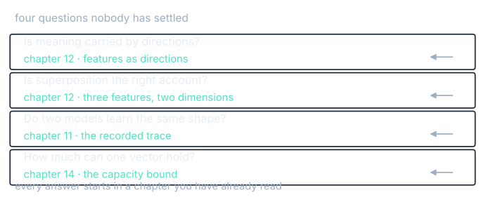
| Question | What would settle it | Where the argument is |
|---|---|---|
| Is meaning carried by directions? | A feature the model can be shown to use whose strength no linear readout recovers | Park, Choe and Veitch 2023 against Engels and colleagues 2024 |
| Is superposition the right account? | A decomposition whose parts the model uses, rather than parts a person finds readable | The sparse-autoencoder papers and their critics |
| Do two models learn the same shape? | Agreement that survives when the two models saw different training data | The Platonic Representation Hypothesis and the measurements around it |
| How much can one vector hold? | A bound stated on ranking rather than on scores, measured on real corpora | Weller and colleagues 2025, and the sign-rank literature behind it |
Is the linear representation hypothesis true?
The linear representation hypothesis is the claim this whole book has been leaning on: a feature the model uses is a direction, and the amount of it present at a position is the dot product with that direction. Chapter 12 built a probe that way. Chapter 13 moved a point along a direction and watched the output distribution move with it.
The evidence for it is that the trick keeps working. Add a direction to the stream and the distribution moves the way the geometry predicts, at the strength it predicts. In the toy, the probe direction flips the top word from coffee to tea at a strength of 1.414, and that number was computed before it was measured. People do the same to real models and get the behavior they aimed for.
The evidence against it is that some things a model tracks are not straight. Engels and colleagues found features that live on a circle rather than along a line: the day of the week, the month of the year. A circle has no single direction that reads position on it, because going far enough in any direction brings you back. Engels and colleagues found such circular features for particular quantities in particular models; nobody has shown they are the rule. A linear probe will find something on such a feature, and what it finds will be a chord across the circle and will be wrong at the ends.
Evidence against it would be a feature the model can be shown to use whose strength no linear readout recovers. The circular features are the strongest case so far. Both sides: Park, Choe and Veitch, The Linear Representation Hypothesis and the Geometry of Large Language Models (2023), and Engels and colleagues, Not All Language Model Features Are One-Dimensionally Linear (2024).
Is superposition the right account?
Chapter 12's three features in two dimensions sit 120 degrees apart and read −0.500 on each other. That arrangement is the standard story for how a model with a few thousand dimensions can track many more than a few thousand things: pack the directions closer than right angles and pay for it in interference.
The current tool for unpacking it is the sparse autoencoder, which learns a large set of directions and a rule that only a few are on at any position. Run it on a real model and you get directions a person can read: one fires on legal language, one on the Golden Gate Bridge, one on code about to raise an error.
There is a second gap. The 120-degree arrangement is the worst case, and the whole design pays off only because the worst case is rare. That turns on sparsity: if one of the three features is active at a time, the interference is the −0.500 reading on the two that are absent and nothing more. Taken as the normal case, chapter 12's crowded picture makes superposition look like a bad design; sparsity is what makes the trade pay.
The papers: Elhage and colleagues, Toy Models of Superposition (2022), then Towards Monosemanticity (2023) and Scaling Monosemanticity (2024).
Do two models learn the same shape?
Take chapter 11's thirteen recorded states and call them version A. Make version B by turning the whole set 30 degrees, scaling it by 1.200, and nudging one state. Read off coordinates and nothing matches. The right question is whether one set is the other set turned around, and it has a standard form.
$$\min_{\mathbf{R}^{\top}\mathbf{R} = \mathbf{I}} \lVert \mathbf{B} - \mathbf{A}\mathbf{R} \rVert_{F}$$In words: search over every rotation $\mathbf{R}$ for the one that, applied to set $\mathbf{A}$, leaves the smallest total gap to set $\mathbf{B}$. The condition $\mathbf{R}^{\top}\mathbf{R} = \mathbf{I}$ is what makes it a rotation and not a stretch, so the fit is allowed to turn the set and nothing else. The answer has a closed form, and the method is called orthogonal Procrustes.
Run it on the two sets and it recovers 29.239 degrees where 30.000 was planted, and a scale of 1.211 where 1.200 was planted. The residual is 0.678, which is 0.006 of version B's spread, and one state carries almost all of it, because one state is the one I moved.
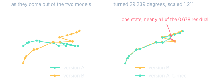
So two versions can agree completely and share no axes at all, which is why comparing coordinates between versions is a mistake. The measurement that survives a rotation is neighbor overlap: for each point, take its $k$ nearest in one version and its $k$ nearest in the other, and count the names on both lists.
$$\frac{\lvert N_k^{(1)}(i) \cap N_k^{(2)}(i) \rvert}{k}$$In words: how many of point $i$'s $k$ nearest neighbors in version one are also among its $k$ nearest in version two, divided by $k$. A rotation does not change who is near whom, so this number does not care which axes either version chose.
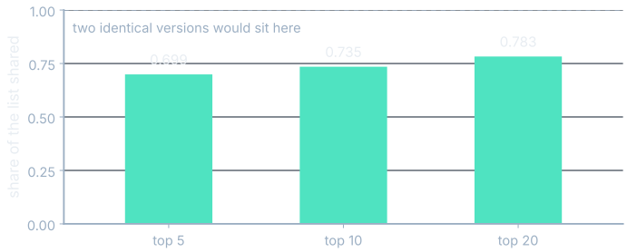
Points in eight dimensions, one version turned and given a little noise, and the top-5 lists share 0.699 of their names. Top-10 share 0.735 and top-20 share 0.783. The rise is arithmetic, because a longer list is easier to overlap, so report the $k$ every time.
The claim that models converge on one shape as they get larger has a name and a paper: Huh and colleagues, The Platonic Representation Hypothesis (2024). It is a hypothesis with evidence behind it, and the measurement it needs is the one above.
How much can one vector hold?
Chapter 14's bound is the cleanest result in these two acts and the easiest to overstate. A bi-encoder scores a query against a document by a dot product, so the score matrix is one thin matrix times another and its rank cannot exceed the dimension. The three-by-three target there has determinant 21.000, so it has rank 3 and no two-dimensional bi-encoder produces it.
What the bound covers is scores. Retrieval needs an order, which is a weaker demand, and chapter 14 measured the gap: two dimensions got the ordering right in 521 of 20,000 random draws even though the exact scores were out of reach. The quantity that governs ordering is the sign-rank, and it can be far larger than the rank.
The open part is empirical. Nobody can tell you, for a real corpus and a real query distribution, how many dimensions the ordering needs. Answering that is what it would take to size an index on purpose rather than by trying 384 and then 768.
The paper is Orion Weller, Michael Boratko, Iftekhar Naim and Jinhyuk Lee, On the Theoretical Limitations of Embedding-Based Retrieval (2025).
Experiment 1: steering a small open model
Three experiments, all of which run on a laptop in an evening.
| Experiment | What you need | What to measure | The control | Roughly how long |
|---|---|---|---|---|
| Steering | A half-billion parameter open model, a laptop, thirty contrast pairs | The output distribution at one prompt, before and after | A random direction of the same length, and the same strength on an unrelated prompt | An evening |
| Probing | The same model, a few hundred labeled sentences | Accuracy on held-out sentences at each depth | The same training run on shuffled labels, a thousand times | An evening |
| Version drift | Two embedding models, 200 sentences | Neighbor overlap at 5, 10 and 20, and the Procrustes residual | The same model against itself with the text lightly reworded | An hour |
The steering method is three steps. Write thirty contrast pairs, short prompts that differ in one property and agree on everything else. Run both halves through the model, take the activations at one layer, and subtract the mean of one set from the mean of the other; that difference is your direction, built the way chapter 12 built its probe. Then run a fresh prompt, add the direction to the residual stream at that layer with a strength you choose, and read the output distribution.
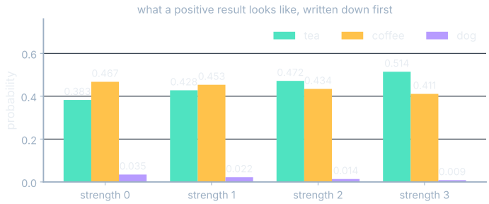
Before you run it, write down what a positive result looks like. Chapter 13's toy gives the shape: as the strength climbs from 0 to 3, tea goes 0.383, 0.428, 0.472, 0.514 and coffee goes 0.467, 0.453, 0.434, 0.411. A smooth move in the direction you aimed at, with the ordering flipping in the middle.
Two controls, and the run is worth nothing without them. Build a random direction of the same length and add that instead: if the distribution moves as much, you have measured what happens when you disturb a residual stream and your contrast pairs did no work. Then take the same direction and strength to a prompt that has nothing to do with the property. If that one moves too, you have found a way to break the model rather than a way to aim it.
The method: Turner and colleagues, Steering Language Models With Activation Engineering (2023), with the wider framing in Zou and colleagues, Representation Engineering (2023).
Experiment 2: probing, with the control
A probe is a small classifier trained on a model's internal states. Label a few hundred sentences for some property, run them through the model, keep the activations at one layer, fit a straight boundary, and report how often it is right on sentences it never saw. Chapter 12 did this by hand: a difference-of-means direction, a threshold at zero, 0.962 accuracy over 26 states. Split the data before you look at it, and report per layer, because where in the depth a property becomes readable is more interesting than whether it is readable at the end.
Then run the control, which is the part people skip. Shuffle the labels so they carry no information at all, train the same probe on the shuffled labels, and see how well it does. On chapter 12's 26 states, over 2,000 shuffles, the mean accuracy was 0.601, the 95th percentile 0.731, and the best of them 0.808.
Two things the control does not cover. A probe finding a property does not show the model uses it, which chapter 12 made with its own numbers. And a big enough classifier learns anything, shuffled labels included, so the control has to use the classifier you used for real.
The probe bench below runs this same shuffle-the-labels control on the twenty-six recorded states from the chapter that built it.
The method: Alain and Bengio, Understanding intermediate layers using linear classifier probes (2016). The control: Hewitt and Liang, Designing and Interpreting Probes with Control Tasks (2019), with the failure modes collected in Belinkov, Probing Classifiers: Promises, Shortcomings, and Advances (2022).
Experiment 3: drift between two model versions
This one runs on the corpus from chapter 9, and I have already run it. The same 10,000 Wikipedia intros, embedded twice: once with all-MiniLM-L6-v2 and once with bge-small-en-v1.5, both 384 dimensions, both permissively licensed, with ids, licenses, pooling and file checksums in versions.json beside the data.
Ask first how far apart the two versions put the same article. Take one article's vector from each model and read the cosine between them. Over all 10,000 the mean is 0.2339. Two models given the identical sentence, and the answer sits nearer to a right angle than to agreement.
Now fit the rotation. One orthogonal Procrustes fit over the whole corpus raises that mean cosine to 0.5809, with a residual of 91.55 over the 10,000 points. The rotation explains a lot and nowhere near all of it, so these two models are not one rotation apart the way the toy versions were.
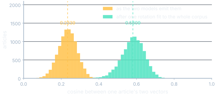
Coordinates were never the thing to compare. Compare the neighbor lists instead.
| Measure | Sample | Value |
|---|---|---|
| Cosine between one article's two vectors | all 10,000 | 0.2339 |
| The same, after one whole-corpus rotation | all 10,000 | 0.5809 |
| Top-10 neighbor lists, shared over combined | 20 fixed articles | 0.2637 |
| Neighbor overlap at 5 | 300 queries | 0.361 |
| Neighbor overlap at 10 | 300 queries | 0.367 |
| Neighbor overlap at 20 | 300 queries | 0.388 |
0.361 of the top five, across three hundred queries. Over the twenty sample articles the top-ten lists share 0.2637 of the names they mention, and one of the twenty, an article about triangular gimbap, scores 0.0000: its ten nearest under one model and its ten nearest under the other have nobody in common.
How to not fool yourself
- Write the prediction down first. The steering figure was drawn before any model was touched: 0.383 rising to 0.514 as the strength goes from 0 to 3. A prediction written afterward fits whatever happened.
- Run the control, with the same classifier. Shuffled labels on 26 states reached 0.808 accuracy by luck. Your result has to clear the luck, and the luck gets better as the dataset gets smaller.
- Compare orders, never coordinates. The same article in two versions sits at cosine 0.2339 and the versions are still useful. Coordinates are a choice of axes. Neighbor lists are not.
- Say which measure and which sample, in the same sentence as the number. This page quotes 0.2637 over 20 articles and 0.361 over 300 queries, and they describe the same disagreement counted two ways.
- Report the part you did not explain. The toy alignment left 0.006 of version B's spread unexplained and it sat on one state. The real alignment left a residual of 91.55 and it was spread everywhere. Those two situations need different next steps, and only the residual tells them apart.
A sixth is more a habit than a rule. When a corpus-level number says nothing happened, look at the per-item numbers before believing it. Chapter 15's drift check has the corpus centroid at a cosine of 0.999, which reads as calm, while one document underneath it moved to 0.979.
Where you'll meet this
- Reading a paper. An interpretability result now comes apart into the claim, the geometry it assumes, and the control. If the control is missing you know which one, and roughly how much accuracy a shuffled run gets for free at that sample size.
- An embedding upgrade at work. When somebody proposes swapping the embedding model, the question is what happens to the neighbor lists, at which $k$, on your queries. The measurement takes an afternoon.
- Your own first experiment. The three above are small, cheap, and produce a number somebody could argue with.
What you now know
- Four questions in this field are open, and each is stated in the vocabulary of an earlier chapter: directions, superposition, shared shape, and capacity.
- The linear representation hypothesis is the claim that a feature is a direction and its strength is a dot product, and the circular features found in real models are the strongest case against it so far.
- Sparse autoencoders find directions that are sparse and readable, and whether those are the directions the model uses is the open part rather than the settled one.
- Two versions can agree up to a rotation and share no axes: orthogonal Procrustes recovered 29.239 degrees where 30.000 was planted, leaving 0.006 of the spread unexplained and almost all of that on one state.
- Two real embedding models put the same article at a cosine of 0.2339, share 0.361 of their top-five neighbors, and one article in twenty shared nothing at all, so coordinates are never the thing to compare across versions.
- Steering, probing and drift each fit on a laptop, each has a prediction on this page saying what a positive result looks like, and each stands or falls on its control: shuffled labels on 26 states reached 0.808 accuracy by luck.
Where to go next
That is the end of this book. You started with a list of numbers read as an arrow and finished with the open problems, and the thing you now know exists is the linear representation hypothesis, along with the fact that you can run the experiment that would test it on your own machine tonight.
Four books sit alongside this one, and each answers a question this one left standing. How LLMs Actually Work is the machine these geometries live inside, from attention through sampling to why a model ever says something false. AI/ML from the Ground Up is the wider field, where a model is a fitted function and a language model is one kind. Training a Model, All the Way Down is where the positions in this book came from, one gradient step at a time. How AI Makes Images takes the same geometry into pictures, where the point you are moving is an image.