A Layer Is a Matrix

The wire is a number

A neural-network drawing can have enough connections to look like a machine made of spaghetti. What would we actually save to disk? We can gather every connection into a matrix, give each output its own bias, and write down the recipe that turns inputs into outputs. The picture then becomes a readable inventory.

We will use the matrix [[1,−1,0],[0,1,1]] and bias [0,0]. This is the output layer of the small model we will follow through several chapters. A weight is a multiplier controlling one input’s contribution. A layer is a set of outputs computed together by one stage. The same input can contribute to several outputs using different weights.

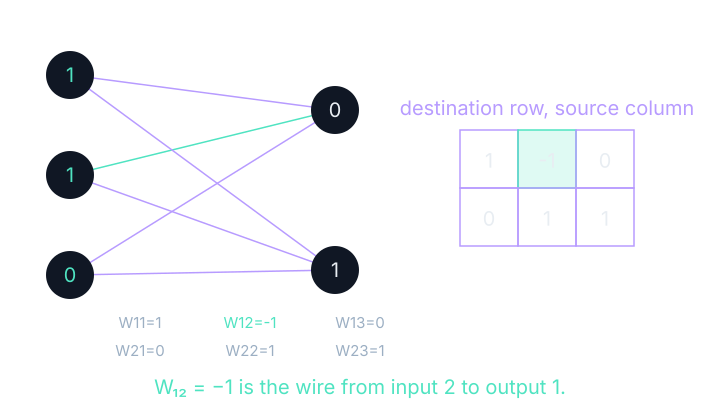
The matrix row names the destination output; the column names the source input. Follow the connection from input two to output one. It is exactly W₁₂=−1, the second entry of the first row. The wire and cell are two drawings of one parameter. A zero entry is still part of the table, even though its connection contributes nothing for the current parameter setting.

A positive weight makes a positive input contribute positively to that row’s sum. A negative weight reverses that contribution. This does not make one connection helpful and another harmful: the task determines which combination is useful. We must calculate the whole output before interpreting its role.

Notice that the same input appears in both calculations. We have not divided the input list between the outputs; each output receives all three entries. This is why this kind of layer is called dense: each destination has a stored multiplying weight for every source input. A particular stored weight may happen to equal zero without changing the layer’s shape.

Warp it, shift it, then bend it

A layer can do more than warp and shift a grid. It can apply an activation, a function after the weighted sum that changes how the result responds to its input. To see the effect without adding more dimensions, return to the original two-coordinate lattice. First leave its warp as the identity, then shift it by (1,−1), then bend each coordinate separately.

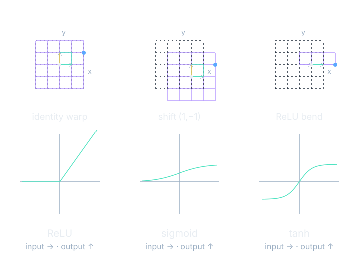
ReLU means rectified linear unit: it returns the larger of zero and its input. The selected point (2,1) becomes (3,0) after the shift, and stays (3,0) after ReLU. Points whose shifted horizontal coordinate is negative land on the vertical axis. Points whose shifted vertical coordinate is negative land on the horizontal axis. Several different original points can now have the same result.

For our fixed model, the internal layer uses tanh and the output layer is unsquashed. Let h name the vector of internal outputs, W the layer’s weight matrix, x its input vector, and b its bias vector. Applying tanh to a vector means applying it to each entry separately, after the matrix multiplication and addition.

In words: multiply and add, include the bias, then apply hyperbolic tangent to every output.

To compare a second activation, use a scalar z for one weighted sum before the bend. The expression e raised to −z is an exponential, not multiplication by a variable named e. Sigmoid’s denominator stays positive, and the resulting fraction approaches its two limiting values smoothly.

In words: the sigmoid divides one by one plus the exponential of the negative input.

Without a bend between layers, repeated linear maps can be combined into one matrix, and repeated affine maps into one matrix plus one bias. Adding more of those stages would change the calculation’s organization without giving it a new kind of shape. A nonlinear activation breaks that restriction. That is the reason for the bend; it earns its place by changing what the model can represent.

A model is a list of parameter arrays

A hidden unit is an internal output between the original input and the final prediction. The width of a layer is its number of units. Depth counts successive learned layers. A parameter is a stored value that training may change. Both multiplying weights and added biases are parameters; forgetting the biases gives the wrong inventory.

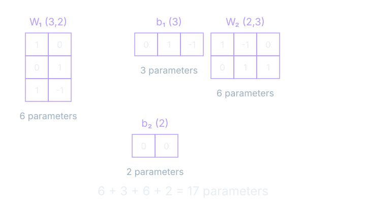
Suppose a layer receives n_in input entries and produces n_out output entries. Each output needs one multiplier per input, so the weight table has n_in×n_out entries. It also has one bias per output. Those symbols count sizes, not particular values. Changing the input from (1,1,0) to another three-entry vector does not change this count.

In words: one multiplying weight per connection, plus one bias per output.

We can read the saved shapes in order: (3,2), (3), (2,3), (2). The first pair belongs to the hidden layer, and the second pair belongs to the output layer. A bias vector’s length matches the number of output rows in its partner matrix. That shape relationship is a useful consistency check before we perform any arithmetic.

The count describes this model’s stored numbers, not all memory needed to train it. Training also keeps intermediate results and derivatives, and an update rule may keep additional state. We will name those quantities when we need them. For now, the ledger tells us exactly which values constitute the model’s learned parameter inventory.

See it move

Select W₁₂ in the output-layer view and change it from −1 to 0. Keep the input (1,1,0) and the other values fixed. The first weighted sum should change from 0 to 1, while the second remains 1. Reset before trying another alteration, so each observation has one identifiable cause.

Try changing a bias instead. Every input presented to that output receives the same added shift. Then switch the activation while leaving the weights untouched. The weighted sums remain the same, but the activation outputs can change. The inspector displays both quantities so that a changed bend cannot masquerade as changed matrix arithmetic.

A wiring diagram is helpful for following one contribution. A matrix table is better for seeing all parameters without crossing lines. Use both views as needed, keeping the selected row and column attached to the same connection. What matters is the numerical relationship, not which drawing style feels more familiar.

Where this shows up when you train

A saved parameter export is an inventory of numbers and shapes. The architecture is the recipe that says how to use them: which arrays multiply, where biases are added, and which activation follows. Training usually changes the parameter values while keeping that recipe fixed for a run. The trained model is therefore more than an unlabeled list of numbers.

We can now connect a parameter edit to a visible consequence. A cell changes a contribution, a row changes an output, and an activation changes the bend after the sum. Next we will ask which pieces of this recipe can be calculated at the same time, and which pieces must wait for earlier results.

Where we’re headed

Next we will count which operations can run together and which must wait. Continue to the next chapter.