You are inspecting a model export and a familiar word suddenly stops being clear. Was that shape counting samples or features? Was the checkpoint the best score or an actual saved state? This reference brings the terms back to their first explanations, where the diagrams and worked values give each definition something concrete to attach to.
Search by a term or an available alias, then follow its first-explanation link. The entries below are generated from the inline definitions in the training chapters. Their wording is the actual tooltip text, not a new definition inferred from a heading. When a later chapter refines a term’s context, that refinement can appear with its own source link. The earliest definition remains the entry’s starting point.
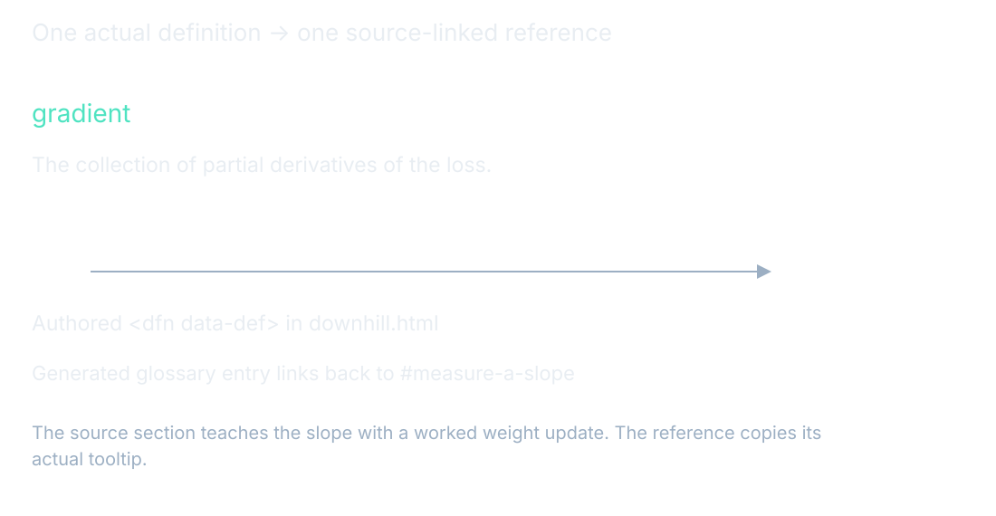
A glossary entry points back to where the idea was taught.
A short definition helps recover a word; the source chapter helps recover the operation. For “gradient,” return to the individual slopes and the weight update. For “shape,” return to the array and its axes. A term is most useful when you can identify the object in a real computation, give its units or dimensions, and say what operation consumes it next. That is why these links return to teaching sections rather than a disconnected list of synonyms.
The symbol stands for an object
A symbol identifies an object or operation; its typography helps tell us which. Bold lowercase letters denote vectors, while bold uppercase letters denote matrices. Plain subscripts name individual entries. The distinction matters when an export contains many arrays: a single weight value and the matrix containing it participate in different descriptions of the same computation. Neither notation changes the numbers stored in the file.
Notation identifies the object and the address of its entries.
The notation table below is generated from the book’s shared notation document. Read a symbol with its local context. Theta can denote all model parameters in a training objective, while an angle in an earlier geometry example also used theta with that meaning explicitly stated. In training, eta is the learning rate and sigma denotes sigmoid. We spell tanh and ReLU explicitly, keeping different activations distinguishable.
Object
Notation
Read aloud
scalar
italic lowercase
"a number x"
vector
bold lowercase
"the vector v"
vector components
subscripts
"v-one, v-two"
column vector literal
bmatrix
"the vector two-one"
matrix
bold uppercase
"the matrix W"
matrix entry
W_{ij}
"the entry in row i, column j"
dot product
center dot
"v dot u" — mint vector FIRST, see rule 8
vector length / norm
\|\mathbf{v}\|
"the length of v"
angle between vectors
\theta
"theta"
cosine similarity
\cos\theta
"the cosine of the angle"
function
f(x)
"f of x"
exponential
e^x
"e to the x"
natural log
\ln x
"the natural log of x"
derivative
\frac{df}{dx}
"the derivative of f with respect to x"
partial derivative
\frac{\partial L}{\partial w}
"the partial derivative of the loss with respect to the weight w"
gradient
\nabla L
"the gradient of the loss"
sum
\sum_{i=1}^{n}
"the sum over i from one to n"
probability
p(x)
"the probability of x"
conditional prob.
p(\text{next} \mid \text{context})
"probability of the next token given the context"
loss
L or L(\theta)
"the loss"
model parameters (all of them)
\theta
"theta — the parameters"
a single weight
w
"a weight"
learning rate
\eta
"eta, the learning rate"
sigmoid (LLM/AIML only — banned in `diffusion/`, see Cross-site collisions)
temperature (LLM/AIML only — see Cross-site collisions)
T
"temperature"
embedding dimension
d (LLM site: d_{\text{model}} once introduced)
"d, the number of dimensions"
vocabulary size
V
"V, the vocabulary size"
context length
n tokens
attention matrices
\mathbf{Q}, \mathbf{K}, \mathbf{V}_{\!a} — NOTE: attention value matrix written \mathbf{V}_{\!a} ONLY if vocabulary V is in scope on the page; otherwise plain \mathbf{V} with a sentence noting it is unrelated to vocabulary size
\{(x^{(i)}, y^{(i)})\}_{i=1}^{N} — introduce gently; prefer "our N examples" in prose
training mean (training/data-into-tensors only)
m
"m, the mean computed from training rows"
training standard deviation (training/data-into-tensors only)
s
"s, the standard deviation computed from training rows"
prediction
\hat{y}
"y-hat, the model's guess"
A matrix and one of its entries
Let W be the identity matrix [[1,0],[0,1]] and x be the vector (1,2). The first output is 1×1+0×2=1. The second is 0×1+1×2=2. Thus this matrix leaves the input unchanged. The mathematical entry W₁₂ is the first row, second column, which contains zero. In Python or JSON the same entry is [0][1], because code indexing starts at zero rather than one.
In words: this identity matrix leaves the input vector unchanged.
Return to containers and indices for the address convention, or space that stretches for the matrix’s action on a point. A two-by-two identity is also a useful first check of a new calculation: if a supposed identity transformation changes (1,2), inspect the axis order and multiplication rule before trusting a more complicated example.
Find the idea in the workflow
The workflow map begins with containers because every later stage receives and returns shaped numbers. A transform changes those values. A forward pass produces predictions, a loss grades them, a gradient describes local sensitivity, and an update changes the parameters. The dashboard displays measurements from that process. Architecture choices change the arrangement of operations, while data and evaluation choices determine what the measurements mean.
The definitions connect back to one continuous training workflow.
Each node returns to the chapter that owns that stage of the story. The arrows show prerequisite direction, not a claim that every software program executes all chapters in order. For example, we choose a data split before training even though the book first explains training with fixed samples. The map is a reading route through ideas; the training-loop diagram is a route through a computation. Both are useful when their purposes stay clear.
Use that small experiment to separate three questions. What are the values? How are they arranged? Which axis has which meaning? Two arrays can have equal counts yet different shapes, and two equal shapes can assign different meanings to their axes. A transpose, a flattening operation, and a changed feature order are therefore not interchangeable descriptions. The source chapters show when each operation is appropriate and how to check it numerically.
The glossary cannot decide whether your model is useful. It can help you express the evidence precisely enough to decide. Name the task, baseline, split, metric, and acceptance criterion. State whether a displayed loss is in-sample, validation, or final test. Explain what one exported weight multiplies and which preprocessing makes that input meaningful. Those statements are stronger than calling a model “trained” without identifying what its score actually measured.
You can also use the reference when explaining a result to someone else. Start with the input and the question the model was trained to answer. Show a prediction and the rule used to score it. Then show the update mechanism and the independent evaluation evidence. The listener need not memorize every symbol to follow the chain if each object is defined where it first becomes necessary. The glossary provides a return path whenever that chain needs a closer look.
What you now know
Definitions point to their first explanation and worked example.
Notation distinguishes arrays from their entries.
The same numeric objects reappear throughout training.
Where we’re headed
You can return to your model export with this reference beside it, or continue to the language-model book to follow the same operations at larger scale. Continue the story.
![Scalar, vector, identity matrix and entry W₁₂; the same entry has JSON address [0][1].](media/glossary-and-notation/notation-objects.svg)