A Number with a Shape

What can twelve numbers look like?

When we open a model’s saved file, we do not find sentences explaining what it knows. We find named collections of numbers. Before we can change those numbers, we need to read the containers: how many entries there are, what belongs together, and how to point to one entry without guessing.

Start with one number, then put a second beside it. A scalar is one number; a vector is an ordered list of numbers. Put two such rows above one another and we have a matrix, a rectangular table. These pictures give us something to point at before the vocabulary becomes more ambitious.

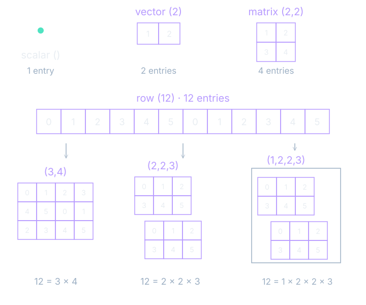
A tensor is a numeric container indexed along axes. An axis is one independent direction in its address: along a row, down a column, or between slabs. The shape lists the length of each axis in order. The rank here counts those axes. A single number has no axis, so we write its shape as the empty pair of parentheses, (). This use of rank differs from matrix rank, which measures independent directions in a transformation.

Our twelve entries are [0,1,2,3,4,5,0,1,2,3,4,5]. Each element is one entry, including repeated values. The two copies of 2 are equal as numbers but occupy different places in the list. We will keep that distinction when we select an entry and change its address.

The shape is part of the meaning. Twelve measurements taken at successive moments and twelve measurements from different sensors could contain identical numbers and still require different treatment. A reshape changes the address system. It does not tell us which physical interpretation is appropriate, and it does not automatically exchange the order of entries.

Every entry has an address

An index is an entry’s address. In a two-by-two table [[1,2],[3,4]], we can locate 3 by saying “second row, first column.” We need both pieces of the address because a row contains several entries. A bare “second” would leave us wondering whether to count rows, columns, or everything in one long sequence.

Now use the two-by-three slab [[0,1,2],[3,4,5]]. We name it the matrix W; bold uppercase letters will name matrices throughout the book. The small letters attached below W identify its row and column. Mathematical addresses on our pages start at one. The address W₂₃ therefore points to the second row and third column, whose entry is 5.

In words: the entry in the second row and third column is five.

A saved JSON list, Python code, and JavaScript use a different starting convention: zero. The code address [1][2] points to the same 5. Nothing about the table changed. Only the counting convention changed. Write the convention beside an address when moving between a diagram and code; this prevents an error that can otherwise look like wrong arithmetic.

A shape such as (3,28,28) now has an ordinary reading: three channels, each with twenty-eight rows and twenty-eight columns. A channel is a separate plane of measurements at the same image locations. The tuple alone does not prove those are the axis meanings; an application must tell us its convention. Another program might put channels last. Matching counts would not make those layouts interchangeable.

The address follows the order of axes. If the channel comes first, the first index chooses a channel. If rows come first, that same index chooses a row. This is why a useful data description contains both axis names and lengths. We will carry those names along the arrows in later computation diagrams.

A picture is a tensor

We can make a small picture with these rules. Imagine a four-by-four grid whose center four cells are bright and whose outer cells are dark. Each location stores brightness: zero for dark and one for bright in this example. An image does not become less of a picture when we write its numbers beside it; we are looking at two views of the same data.

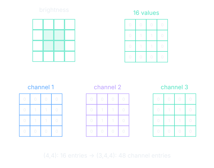
The brightness rows are [0,0,0,0], [0,1,1,0], [0,1,1,0], and [0,0,0,0]. Four rows times four columns gives sixteen entries. A color image can keep three measurements per location. RGB names red, green, and blue image channels. Three copies of our example form shape (3,4,4), with 3×4×4=48 entries. Identical channels would still describe a grayscale-looking image.

The dtype tells us how a number is represented in storage. A byte is a unit of eight binary storage digits. The dtype float32 represents a floating-point number using four bytes. Floating point can represent fractions and a wide range of magnitudes, but only a finite set of values. We will round displayed calculations for readability while keeping more precision inside the interactive examples.

The picture’s visible size on the page is yet another quantity. Enlarging an illustration on your screen need not create more stored pixels. Changing its actual grid from four rows to eight rows does require a rule for creating new values. Keep the container, its storage representation, and its display size separate when you inspect an image dataset.

Rearrange the container

Before changing the shape below, find the selected 2. Predict its address in a three-by-four grid. Read across the original list: flat offsets zero through three fill row zero, four through seven fill row one, and eight through eleven fill row two. Our selected entry therefore becomes the first entry of row two under code indexing.

See it move

Enter (3,4), choose Reshape, and check the selected entry. Then return to (2,2,3) and change only the index convention. The value should stay 2 through both actions. One control changes the arrangement; the other changes the names we give addresses. Neither operation has trained a model or altered a measurement.

Try requesting a shape with a different total count. The control reports the mismatch and offers a separate regeneration action. That distinction matters: reshaping preserves entries, while regeneration makes a new list. A larger shape displays a slice and its full count so the page remains usable; the omitted view is not a claim that the unseen entries disappeared.

Where this shows up when you train

When a training program reports a shape mismatch, start with the named axes. A batch is a group of examples processed together. Adding a batch axis places several image tensors in one larger container; it does not mix their pixels. The batch length tells us how many examples the operation receives together, while each example retains its own channels, rows, and columns.

This is the first habit of the workshop: make the stored object concrete. We can count its entries, locate one value, and explain what each axis means. Once those checks are routine, a model’s weight file stops looking like an opaque blob and starts looking like a collection of inspectable tables.

Where we’re headed

We can read the numbers a model holds. Next we will make a matrix move arrows and an entire grid. Continue to the next chapter.