Choose the task before the model
We have a dataset and a way to turn it into tensors. Now we must choose what the run should optimize and how we will decide when it has done enough. I want those choices written down before a promising curve tempts us to change the question. A training recipe is a set of testable decisions, not a collection of lucky knobs.
A hyperparameter is a choice outside the parameter updates, such as width or learning rate. capacity is the range of patterns a model can represent. A baseline is a simple comparison rule. Before selecting a model size, choose a baseline and a metric on the intended split. A network that fails to improve on a useful baseline has not earned its extra complexity for that task.

The recorded families offer starting examples. Dense layers combine table features; convolution shares rules over image grids; recurrent updates carry state through ordered streams; attention compares token positions; graph layers gather along explicit edges; autoencoders reconstruct inputs. Match classification labels to cross-entropy and numerical or reconstruction targets to squared error when those objectives fit the task. Match the baseline too: majority class, training mean, or persistence of the previous observed value.
Look for a useful rate range
A learning-rate finder is a short run that increases the rate to locate a promising range. That is different from independent trials that each hold a rate fixed. E9 contains the latter: separate fixed-rate experiments. E9b contains one continuous increasing-rate run. We need both the axis labels and the procedure to interpret a curve correctly; a horizontal axis called “rate” does not tell us which experiment happened.
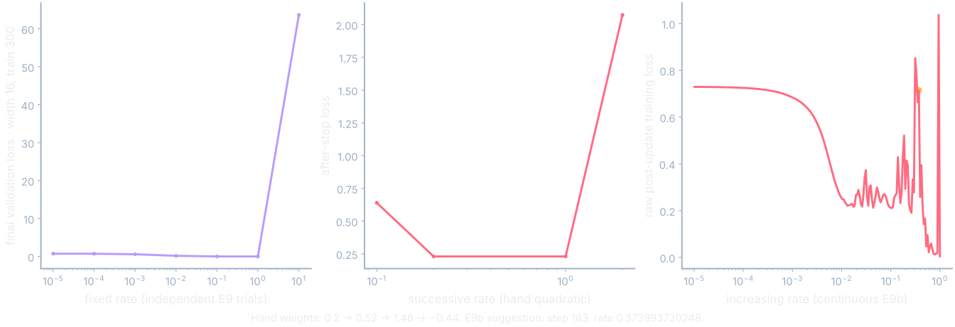
E9b applies 200 increasing rates from 1e-5 to 1 to E3’s model and split using Adam. Its saved heuristic suggests 0.373993730248 at step 183, from media/runs/E9b.summary.json#/values/suggested_rate and /values/suggested_step, with the rule recorded in /meta/headline. The rule minimizes the centered slope of unsmoothed full-training-split post-update loss against log10(rate), excluding endpoints. This is a heuristic for that run, not proof that the suggested rate is universally stable.
An increasing-rate test by hand
Let L(w)=(w−1)², so the gradient is 2(w−1), starting at w=0 and loss 1. Use rates [0.1,0.2,1,2] in that order. First the gradient is −2, so w becomes 0−0.1(−2)=0.2 and loss becomes 0.64. Next the gradient is −1.6, so w becomes 0.2−0.2(−1.6)=0.52 and loss becomes 0.2304. These are sequential steps on one changing weight, not four independent starts.
The larger rates
At w=0.52 the gradient is −0.96. Rate one gives 0.52−1(−0.96)=1.48, with after-step loss 0.2304 again. We crossed the minimum without reducing the loss. The gradient is now 0.96; rate two gives 1.48−2(0.96)=−0.44, whose loss is (−1.44)²=2.0736. That is nine times the preceding loss. The resulting weights are [0.2,0.52,1.48,−0.44]. This hand quadratic does not determine E9b’s suggested rate.
Compare like with like
A fair fixed-rate comparison holds other relevant choices in view. E9 has 84 trials: two families, seven rates, three widths, and two requested data sizes. The requested size is not always the actual size. In particular, E2’s larger request is capped at 48 training rows. Calling it a 300-row experiment would make its comparison with E3 misleading before we even opened the curves.
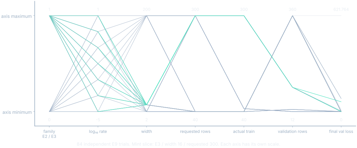
Each line passes through a trial’s family, rate, width, requested size, actual training size, validation size, and final validation loss. These axes use different scales; their vertical alignments do not imply equal units. Filter one family and actual size before comparing rates or widths. A line that looks unusually steep between two axes can result from axis scaling rather than an unusual training event.
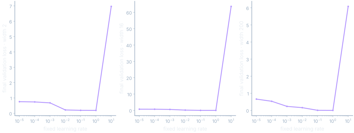
A sorted endpoint table helps locate candidates, while raw curves show how they arrived there. Keep a failed trial’s recorded status and available endpoint; do not fabricate a final value when none exists. Training-loss minima alone can reward memorization. Validation supplies the development criterion, but repeated selection using it is still development. These coupled small trials do not establish causal parameter-importance rankings.
Choose constraints before seeing the final score
regularization refers to choices that discourage fitting details that fail to transfer. dropout randomly masks intermediate activations during training. A seed initializes pseudorandom choices such as masks, shuffling, or weights. reproducibility means recording enough procedure, data, and environment information to repeat the result. The seed is useful, but it is only one part of that record.
Inverted dropout
Take hidden values (1,2), a keep fraction of 1/2, and a sampled mask (1,0). Inverted dropout keeps the first value and divides it by the keep fraction, while dropping the second: (1×1/(1/2),2×0/(1/2))=(2,0). Inference uses the full (1,2). The scaling preserves the expected contribution over masks, not the exact contribution of this particular mask. This hand calculation illustrates the operation; it is not a claim that every recorded family used dropout.
After development, evaluate the final test once under the agreed rule. If the result leads us to change the model, that test has influenced development and no longer serves the same untouched role. Keep the full decision record, including unsuccessful choices. Recording only the winning seed or best endpoint hides how much selection occurred and can make a repeat look inexplicably worse.
Where this shows up when you train
The designer starts from planar binary classification and an E3 sweep slice with width sixteen and requested size 300. Narrow the rate range using either the plot’s brush or the numeric controls. The companion table and raw curves update together. Then edit the hand rate sequence and inspect each new weight and loss. Those local calculations are explicitly separate from the fixed measured trial endpoints.
What you now know
- The task and evaluation criterion determine what to optimize.
- Sweep comparisons must hold relevant settings and actual data size in view.
- A seed and a stopping rule are parts of the run’s reproducible record.
Where we’re headed
Next we will decide whether the trained model did anything useful beyond the baseline. Continue the story.