From a loop to a reduction
Suppose we have a correct little program made of loops, but it runs slowly. How do we turn it into array operations without changing its answer? We will work through an average, a distance table, and an image blur. For each, we will identify one output, write its arithmetic, and decide which axis gets combined.
Start with [1,2,3]. A loop can accumulate 0+1=1, then 1+2=3, then 3+3=6, and divide the total by three. The answer is 2. A reduction combines entries along an axis, as this sum does. It replaces several input entries with one result for the group being reduced.
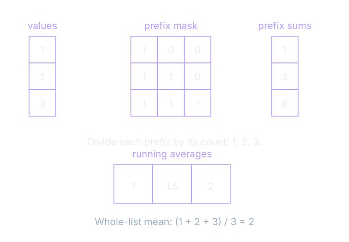
A whole-list mean and a running average have different output shapes. The whole-list mean returns one number. The cumulative running average returns one number for every prefix: [1,(1+2)/2,(1+2+3)/3]=[1,1.5,2]. A prefix is the initial portion ending at a particular position. The final entries agree, but the earlier outputs are additional information.
The loop’s changing accumulator makes the sequential dependency visible. Addition allows another organization, provided we account for floating-point rounding. A prefix scan computes the accumulated result for every initial portion of a list. It is a useful operation in its own right, not an instruction to build an enormous matrix full of zeros and ones.
A matrix that explains every prefix
Multiply the lower-triangular mask [[1,0,0],[1,1,0],[1,1,1]] by (1,2,3). The rows give 1, 1+2=3, and 1+2+3=6. Divide those entries by (1,2,3) entry by entry. The running averages are (1,1.5,2). The zeros state which later inputs each prefix excludes.
This dense mask explains the index pattern, but it wastes storage as the list grows. The practical implementation can use a scan with much less temporary storage. This is our first distinction between a mathematical representation and an implementation choice: showing an operation as a matrix does not require a program to materialize every cell of that matrix.
One point against every other point
Next consider six points: A=(0,0), B=(1,0), C=(2,0), D=(0,1), E=(1,1), and F=(2,1). We want the distance between every pair. Each output cell has two point indices: a row point and a column point. One cell’s answer is independent of the others once the original coordinates are available.
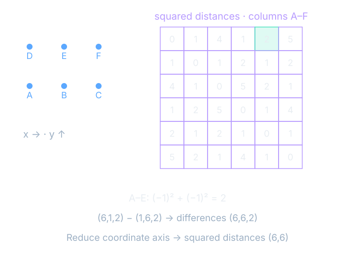
To broadcast arrays is to align compatible axes and conceptually repeat values across them. The operation can often reuse storage instead of physically copying every repeated input. Here one copy of the point list supplies the row-point axis and another supplies the column-point axis. A third axis holds the two coordinate differences needed for each pair.
If X has shape (6,2), the expression X[:,None,:] exposes shape (6,1,2), while X[None,:,:] exposes shape (1,6,2). A colon means to select every entry along that existing axis. None inserts an axis of length one. Subtracting these views produces the conceptual pair-and-coordinate shape (6,6,2).
Inspect A against E
The difference between (0,0) and (1,1) is (−1,−1). Squaring gives (1,1); adding gives squared distance 2; taking the square root gives distance √2. From A, all six squared distances are [0,1,4,1,2,5]. The table in the figure deliberately labels squared distances so that its integers are not mistaken for ordinary lengths.
Let Dᵢⱼ name the distance from point i to point j. The coordinate index k visits the two coordinates inside each pair. The point indices survive into the output table; the coordinate index disappears because we reduce it by summing. That is the pattern we want to recognize before choosing a library expression.
$$ D_{ij}=\sqrt{\sum_k(X_{ik}-X_{jk})^2} $$In words: subtract the coordinates, square the differences, add them, then take the square root.
A six-by-six-by-two temporary is small. The same pattern on a much larger point set can create an expensive intermediate. An algebraic alternative computes squared distances from dot products and squared norms, avoiding the full difference tensor. The comparison is therefore about arithmetic and memory together, not whether the source code contains fewer lines.
The image operation behind the loop
Our third program slides a local average over an image. Use a five-by-five input whose every row is [0,0,3,0,0]. An image kernel is a shared local array of weights applied to patches. This differs from the device program called a kernel in the preceding chapter. The same word names two related but distinct objects.
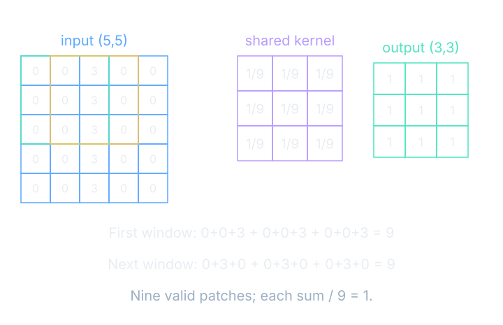
The averaging image kernel is three by three, with 1/9 in every entry. Padding would add border entries around the image; here there is no padding. Stride is the amount the window moves between outputs; here it is one cell. A five-cell side admits three valid positions for a three-cell window, so the output is three by three.
Each output reads its own patch of the original image. Neighboring outputs share many input pixels, but neither requires the other’s output. A program that overwrites the original image while sliding would change this dependency: later windows could read already-blurred values. Keeping input and output separate preserves the operation we intend to express.
The first two windows
The first sum is 0+0+3+0+0+3+0+0+3=9, divided by 9 to give 1. The next is 0+3+0+0+3+0+0+3+0=9, divided by 9 to give 1. The same central stripe lies inside every valid window, so all nine output cells equal 1.
Conceptually flatten each three-by-three patch into nine entries and stack the nine patches into rows. Each row’s dot product with the flattened averaging kernel gives one output. We have exposed the same repeated local computation as a tensor operation. An efficient implementation may gather patches implicitly; the conceptual stack does not prove that all patch values must be copied into a new array.
Watch the same cell in both programs
To vectorize is to express a calculation as array operations instead of one interpreter-level operation per element. Contiguous memory means neighboring logical entries occupy neighboring storage locations under a specified layout. Both ideas can help a library process many entries efficiently, but neither alone guarantees that a rewritten program is faster.
See it move
Begin with blur. Step the loop and select its corresponding output cell. Read the full nine-term sum before requesting all independent outputs together. Then switch to distances and inspect the coordinate reduction in a selected pair. In average mode, distinguish the whole-list reduction from the prefix output rather than assuming that both return the same shape.
The editable examples are deliberately small enough to inspect. B1b timed larger workloads: 100,000 values for running average, 2,000 two-dimensional points for distances, and a 1024×1024 input for valid three-by-three blur. The measurements below are median-of-five seconds. Their source arrays remain in B1b.json; no timings come from moving the browser’s demonstration cursor.
The transfer-inclusive result changes the interpretation. CUDA compute is faster than the NumPy blur measurement here, while CUDA with transfer takes slightly longer than NumPy. That is a result for this recorded workload and boundary, not a contradiction. The two CUDA intervals include different amounts of work around the arithmetic itself.
Where this shows up when you train
A batch axis repeats examples, while a feature axis contains the values inside one example. A reduction removes the axis whose entries it combines; broadcasting exposes axes over which a calculation repeats. These ideas let us describe data preparation, layers, and losses with the same shape vocabulary. They also make large temporary arrays easier to spot before they exhaust memory.
For each proposed rewrite, name the surviving output axes, the reduced axes, and any intermediate arrays. Check whether every output reads the original inputs. Then time the actual workload with its copying and allocation boundary stated. That sequence gives a performance claim something concrete to rest on.
What you now know
- Vectorizing preserves the arithmetic while changing how work is scheduled.
- Broadcasting pairs compatible axes, and reductions combine an axis.
- A faster-looking animation is not a measured speedup.
Where we’re headed
The next step is choosing the axes before writing the loop. Continue to the next chapter.