Train Your Own Model · Training a Model, All the Way Down

Open the shipped package

We can now train a small model and explain what the resulting file contains. Start with a supplied sample so we can check the path, shapes, and output before changing the data. Then replace the input with your own examples and keep the same evidence: command, split, metric, baseline, and one weight row whose multiplication you can explain.

A command line is a text interface for running a program with arguments. Download trainkit.zip and extract it. Open a terminal in the parent directory containing trainkit/. A path identifies a file or directory relative to that location unless it starts from the filesystem root. The output argument names the directory where this run’s two current files will be written.

Install in a virtual environment

Create a virtual environment with python3 -m venv .venv on Linux or macOS, or py -m venv .venv on Windows. Activate it using source .venv/bin/activate on Linux/macOS or .venv\Scripts\Activate.ps1 in PowerShell. On Linux, run the commands below. On Windows use py -m pip in place of python3 -m pip. These training commands need no GPU.

python3 -m pip install torch --index-url https://download.pytorch.org/whl/cpu
python3 -m pip install ./trainkit

The package pins torch==2.14.0+cpu on Linux and Windows. If the first command selects a newer version, install that pinned version from the same CPU index before installing trainkit. On macOS use python3 -m pip install torch==2.14.0, then install ./trainkit; its non-CUDA wheels do not use the +cpu suffix. The network download is part of your installation, not part of the recorded offline measurement below.

Draw the extracted package directory and a chosen output directory; connect the input CSV/images to the CLI and its separate run.json/model.json outputs. Label observed formats from receipts. — The runner produces a measurement record and a readable parameter export.

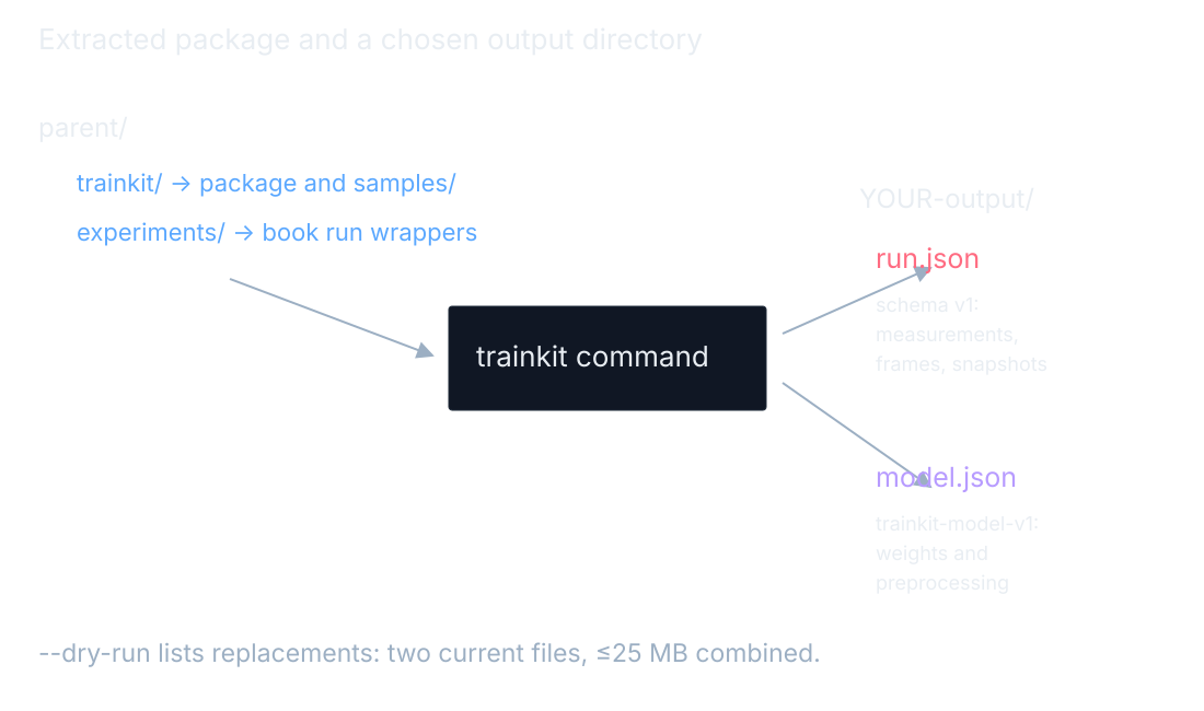
The commands shown next are the exact repository commands recorded during P2, with their recorded output directories. In an extracted installation, use python3 -m trainkit or py -m trainkit in place of the repository’s .venv executable and adjust paths to the samples. Verify your working directory before pasting a relative input path. The downloaded archive includes the package and experiment sources used by the book.

Fit a function and read every update

Begin with the twelve-point function fit. Its model predicts ax+b, so the export holds one multiplying weight and one bias. The small task prints every update’s parameters and gradients. It evaluates the same twelve inputs it trains on; the label “validation” in its output does not turn that into held-out evidence.

Run the recorded fit command

.venv/bin/python -m trainkit fit trainkit/samples/fit.csv --output /tmp/training-p2-evidence/fit

The first printed update is a=0.157576, b=0.200000, grad_a=−1.575758, grad_b=−2.000000. The last exported values are a=1.985458 and b=0.999998. Compare the signs: the negative initial gradients make a positive update when the optimizer subtracts the scaled gradients. The final values approach the sample function’s slope and intercept through the repeated arithmetic we already studied.

Train the sample table

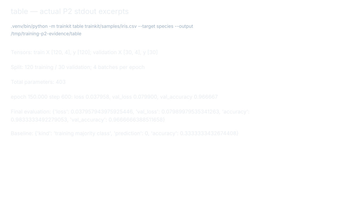
The table command reads four features and a species target from the supplied sample. Check the printed tensor shapes before the losses. Training X is [120,4] with y [120]; validation X is [30,4] with y [30]. The model has 403 parameters and performs four batches per epoch. These dimensions describe this sample only. With your own file, your numbers will differ; the shape’s second number is your feature count after preprocessing. Categorical features expand into one column per training category. The first number counts examples in that split; classification y has one label per example, while regression y has shape [examples, 1].

Render exact table stdout excerpts from command_receipts with labels for tensor shapes, split, parameter inventory, final epoch and baseline. Preserve printed values and clarify decimal fraction versus percent. — This is the actual sample-table output recorded during P2.

Train and compare

.venv/bin/python -m trainkit table trainkit/samples/iris.csv --target species --output /tmp/training-p2-evidence/table

The last printed epoch is 150, step 600: loss 0.037958, val_loss 0.079900, val_accuracy 0.966667. The unrounded final validation accuracy is 0.9666666388511658. The training-majority baseline accuracy is 0.3333333432674408 on the same validation split. The sample model beat that baseline. These are decimal fractions, not percentage literals, and this validation result is not an untouched final test of every dataset we might provide later.

Use the other shipped sample formats

The image and sequence commands reuse the same overall pattern: load, describe shapes, train, evaluate, and export. Their inputs and objectives differ. Keep the task-specific baseline beside each score and read whether higher or lower is better. The figure shows actual transcript excerpts, so we can compare the command and split with the book’s experiment before treating them as the same run.

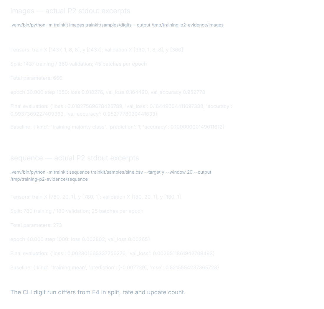
Render exact image and sequence stdout excerpts, each with its sample command and split. Put book E4 and this CLI run in separate labeled contexts. — CLI defaults and book experiment settings produce different runs.

.venv/bin/python -m trainkit images trainkit/samples/digits --output /tmp/training-p2-evidence/images

The image command reports training X [1437,1,8,8], validation X [360,1,8,8], and 666 parameters. Final validation accuracy is 0.9527778029441833, compared with baseline 0.10000000149011612. This CLI run differs from E4 in split, rate, and update count. Its model family and parameter count can match without making its recorded accuracy interchangeable with E4’s endpoint.

Train a sequence window

.venv/bin/python -m trainkit sequence trainkit/samples/sine.csv --target y --window 20 --output /tmp/training-p2-evidence/sequence

This reports training X [780,20,1], validation X [180,20,1], and 273 parameters. Final validation mean squared error is 0.0026511861942708492, against mean-baseline error 0.5215554237365723. Lower is better. The sequence loader uses the target’s history only and ignores other columns. Its windows respect the chronological split, which is why the input count is smaller than the number of raw rows.

Replace the input path and target

Replace the sample path and identify your target before changing anything else. A table needs a header and finite numeric or categorical features, with enough examples per class for the chosen split. Missing, malformed, or nonfinite cells are errors. An identifier that leaks the target can still be syntactically valid, so the loader’s acceptance does not replace the split and feature review from earlier chapters.

A measured house-price regression

Use trainkit table house_prices.csv --target price --output house-output. This measured example uses a synthetic 400-row table with four numeric features and prices in dollars. Its default task detection selects regression. The loader fits the target mean and standard deviation on training rows only, trains on (price − mean) / standard deviation, and converts predictions back to dollars for evaluation. The defaults are 150 epochs, batches of 32, and Adam with learning rate 0.01.

Tensors: train X [320, 4], y [320, 1]; validation X [80, 4], y [80, 1]
Split: 320 training / 80 validation; 10 batches per epoch
0.weight                 [16, 4]                 64 parameters
0.bias                   [16]                    16 parameters
2.weight                 [16, 16]               256 parameters
2.bias                   [16]                    16 parameters
4.weight                 [1, 16]                 16 parameters
4.bias                   [1]                      1 parameters
Total parameters: 369
epoch 150.000 step 1500: loss 113131112.000000, val_loss 122866216.000000
Final evaluation: {'loss': 113131112.0, 'val_loss': 122866216.0, 'rmse': 10636.311014632845, 'mae': 8602.892578125, 'r2': 0.9941526565674457, 'val_rmse': 11084.503416933028, 'val_mae': 8895.0078125, 'val_r2': 0.9933911835403447}
Baseline: {'kind': 'training mean', 'prediction': [395236.625], 'mse': 18592370688.0, 'rmse': 136353.84368619756, 'mae': 117319.1875}
Regression units: loss/val_loss and baseline MSE are target units squared; RMSE/MAE are target units.
Validation R²: 0.993391
beats baseline: yes (by 99.34%)

This excerpt keeps the opening inventory and final evaluation; the CLI also prints each epoch’s loss line. Tensors gives the input X and target y shapes; Split gives the training and validation counts and batches per epoch. Each named weight or bias line gives its shape and scalar parameter count; Total parameters sums them. An epoch counts passes through training examples; a step counts optimizer updates. loss and val_loss are training and validation mean squared error (MSE), in dollars squared here.

Read the metrics and their references

Final evaluation repeats the final losses and adds RMSE (the square root of MSE), MAE (mean absolute error), and R². The val_ prefix identifies validation metrics; unprefixed metrics use training examples. RMSE and MAE are in dollars here. Regression units identifies these units for any target. Validation R² compares the model’s squared error with predicting the validation mean, while the printed Baseline and beats baseline percentage compare it with predicting the training mean on those same validation rows. For R², 1 is perfect, 0 matches the validation-mean reference, and a negative value is worse; it is undefined for a constant validation target. The baseline reports MSE, RMSE, and MAE. Because the two references use different means, the baseline percentage improvement need not equal R² times 100.

beats baseline: yes/no (by x%) compares validation MSE: x = 100 × (1 − model MSE / baseline MSE). A negative percentage means worse; a zero baseline has no defined percentage improvement and cannot be beaten. This run reduced validation MSE by 99.34%. Your result depends on your data. Classification instead prints cross-entropy loss, accuracy/val_accuracy as fractions correct, and the training-majority class prediction and its validation accuracy. The small fit command additionally prints a and b (weight and bias), grad_a and grad_b (their batch gradients before the update), then the full named weights and gradients dictionaries.

Read what the model learned

An export is a saved representation of values and their metadata. Open model.json to inspect the parameters and preprocessing that give those values meaning. Open run.json in the dashboard for training curves and recorded states. The two files have different schemas because they answer different questions. The readable parameter export is not a complete optimizer-resume checkpoint.

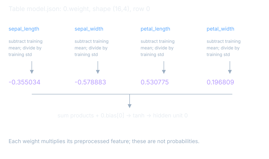
The four observed first-row weights under four input feature slots; labels explain training-standardized features, sum, bias and tanh. Load actual feature names/preprocessing from the table model receipt, not invented feature order. — A weight row specifies how one hidden unit combines its preprocessed inputs.

The inspected table export has format trainkit-model-v1. Its first tensor, 0.weight, has shape [16,4]. The first row is [−0.355034,−0.578883,0.530775,0.196809]. In order, these multiply standardized sepal_length, sepal_width, petal_length, and petal_width. Then 0.bias[0] is added and tanh applied. These four numbers are one hidden unit’s input multipliers, not four class probabilities or four independent feature-importance scores.

.venv/bin/python -c 'import json; m=json.load(open("/tmp/training-p2-evidence/table/model.json")); print("format:",m["format"]); print("parameters:",[(p["name"],p["shape"]) for p in m["parameters"]]); k=m["parameters"][0]["name"]; print("first tensor:",k); print("first row:",m["weights"][k][0])'

Where this shows up when you train

To complete the capstone, keep the command, input and split description, final metric and baseline, first weight row, and a sentence explaining what each row entry multiplies. A completed process alone is not a success claim. If the model misses the intended criterion, use the diagnostic checks from the previous chapter and retain that result in the record.

What you now know

The CLI reports data shapes, parameter shapes and evaluation.
The sample result and the baseline must use the same split.
An exported weight row specifies input multipliers for a unit.

Where we’re headed

The final chapter gathers the terms and notation so we can return to any definition while working. Continue the story.