What shape does it eat?
A list of measurements arrives in time order. We want to predict the next one, and yesterday’s order matters as much as yesterday’s values. How do we reuse a model without pretending that each position is independent? We’ll carry a small numeric state through the list and watch what happens to it.
A sequence is an ordered list of inputs. A time step is one position in that list, which is different from an optimizer step that changes weights. A recurrent network repeats a shared update using the previous hidden state. The hidden state is the vector carried from one sequence position to the next. E5 uses a window of twenty preceding numerical target values to predict the next value.
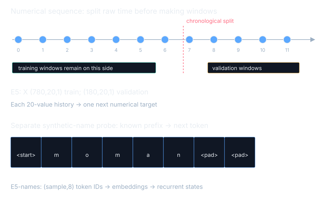
The input axes are sample, sequence position, and feature. For this numerical task the feature axis has length one. We preserve chronological order and construct windows separately on each side of the raw-data split. A window that crossed the split could quietly bring evaluation history into a training example. Shuffling independent training windows later is a different operation from shuffling the time positions inside each window.
A repeated rule carries a state
unrolling means drawing repeated state updates as an ordered chain. There are several visible copies of the calculation, but just one shared set of parameters. The state output of one copy becomes an input to the next. This creates a dependency that a recurrent forward pass must respect: we cannot finish a later state before we have the preceding one.
A gate is a learned mixing fraction controlling retained and replaced state. A gated recurrent unit uses reset and update gates. The reset gate controls the old-state contribution used to construct a candidate; the update gate controls how much old state to keep. E5’s stored parameter rows follow the reset, update, candidate ordering, with separate input and hidden matrices and biases.
Three positions, the same weights
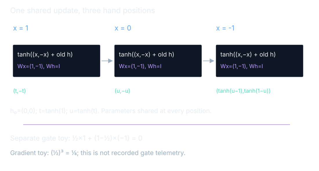
We’ll use a two-unit hand recurrence, keeping the trained gated model separate. Start with hidden state (0,0). The scalar inputs are 1,0,−1. The input weights are (1,−1), the recurrent matrix is the identity, and both biases are zero. Thus each update applies tanh to (x,−x) plus the old state. Every input and weight can be edited in the hand widget.
Three updates with one parameter set
Let t=tanh(1) and u=tanh(t). The first state is (t,−t), because the old state contributes zero. With the next input zero, the second state is (u,−u). With the final input −1, the third state is (tanh(u−1),tanh(1−u)). Evaluating tanh(z)=(exp(2z)−1)/(exp(2z)+1) gives (0.7615941559557649,−0.7615941559557649), then (0.6420149920119997,−0.6420149920119997), then (−0.3434379411684755,0.3434379411684755).
The signs reverse on the last input because the new negative contribution outweighs the retained positive coordinate. Nothing changed in the weights during these three positions. Let bold x at position t be the input vector, bold h the hidden state, and bold W with subscripts x and h the input and recurrent weights. Bold b is the bias. For the separate gate formula, g is the fraction of old state retained:
$$\mathbf{h}_t=\tanh(\mathbf{W}_x \mathbf{x}_t+\mathbf{W}_h\mathbf{h}_{t-1}+\mathbf{b})$$In words: the vector x at position t holds the current input; mix it with the previous state, add the bias, and bend the result. The hand example above has only one input feature.
$$h_{\mathrm{new}}=g h_{\mathrm{old}}+(1-g)h_{\mathrm{candidate}}$$In words: keep the gate’s share of the old state and the remaining share of the candidate.
A gate and a shrinking derivative
With old state 1, candidate −1, and keep-gate 1/2, the next state is (1/2)×1+(1−1/2)×(−1)=0. Keeping more of the old state would pull the result toward 1; keeping less would pull it toward −1. Separately, a local slope of 1/2 repeated through three links returns a derivative of (1/2)³=1/8. The first calculation is a state mixture; the second is a gradient product. Neither supplies measured gate values for E5.
Compare state and prediction while training
The numerical E5 model has an eight-coordinate GRU state and a final linear readout of its last state. The token model adds an embedding and applies its output head at each position. These are different tasks even though both use the same recurrent family. We therefore compare the numerical run to its numerical baseline, and the name run to other models using the same name corpus and split.
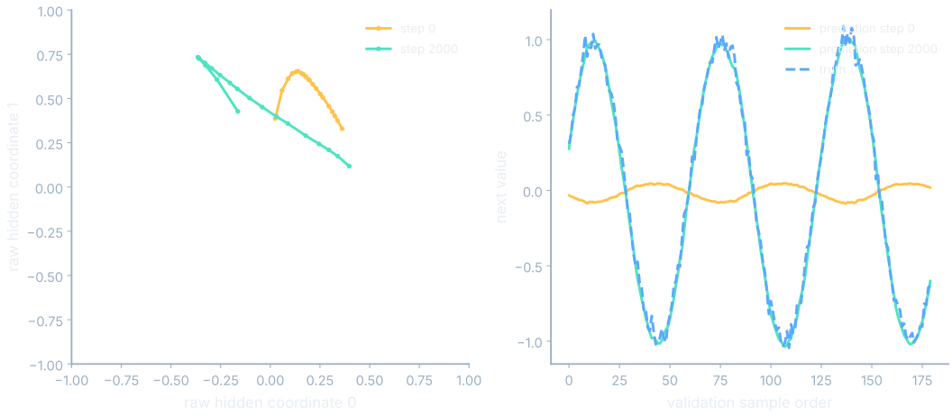
At optimizer step 2000, E5’s training loss is 0.002882 and validation loss is 0.002866. The source is media/runs/E5.summary.json, fields /values/final_loss and /values/final_val_loss, pointing to series index 2000. E5-names has final validation loss 1.325217 at index 2000 in its own summary. The numerical loss and character cross-entropy use different units, so their magnitudes are not a contest between tasks.
Where this shows up when you train
Ordered streams can benefit from a shared state update, especially when the recent past is useful for the next prediction. The relevant question is what history is available at the moment we must answer. A window built using a future observation would make the score easier while changing the real task. Preserve the temporal boundary before considering whether a larger recurrent state might help.
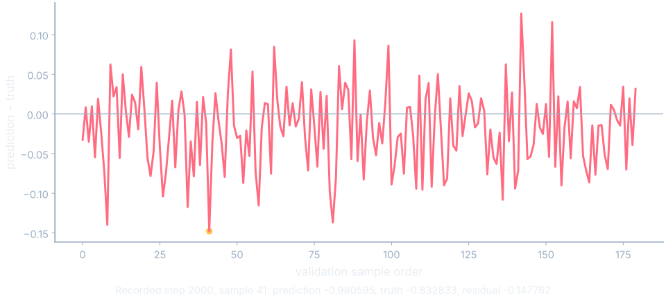
A residual is prediction minus truth. The figure identifies the largest absolute residual among the final saved numerical predictions, using the first index in a tie. It shows the prediction, truth, and their difference at that exact array location. That is an observed failure in this recorded frame; it is not a fabricated “hard sequence.” Selecting another sample in the replay lets us inspect the same arithmetic elsewhere.
What you now know
- A recurrent model applies the same state-update rule along a sequence.
- A gate chooses shares of old and candidate state.
- Recorded predictions reveal what this task did and did not teach.
Where we’re headed
Attention will let each position form its own mixture of other positions instead of relying only on a carried state. Continue the story.