Space That Stretches

Two arrows move the whole grid

What does changing a number in a matrix actually do? We can answer by watching a whole grid move. We already know how to read the matrix’s rows and columns; now each column will tell us where a particular arrow lands, and those two arrows will determine the movement of every point.

Start with (1,0), one step along the horizontal axis, and (0,1), one step along the vertical axis. These are unit arrows: each has length one. We can reach (2,1) by taking two copies of the first arrow and one copy of the second. A linear map preserves that recipe when it moves the arrows. A transform is the rule that sends each input position to its output position.

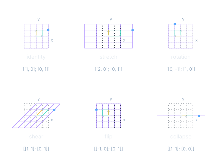
Read the six matrices as movements. The identity [[1,0],[0,1]] leaves both arrows in place. A scale [[2,0],[0,1]] stretches the horizontal direction. The rotation [[0,−1],[1,0]] makes a quarter turn. The shear [[1,1],[0,1]] slants vertical lines. The flip [[−1,0],[0,1]] reverses the horizontal direction. Finally, [[1,1],[0,0]] collapses the plane onto a line.

In every panel the first column gives the new position of (1,0), and the second gives the new position of (0,1). We never assign each point a separate movement. Each point follows from the same two column arrows, so straight grid lines remain straight and parallel lines remain parallel, even when several points collapse together.

A matrix-vector product performs that row calculation once per output. Let the matrix be W, the input vector be x, and the output vector be y. The subscript i selects an output row; j visits each input coordinate. The summation sign means to add the indicated terms as j changes. It is a compact spelling of the arithmetic we just performed.

In words: each output is the sum of one matrix row multiplied entry by entry with the input.

One row gives one output

One row of W behaves like a short list of multipliers. A dot product multiplies matching vector entries and adds the products. Before we use it as an arithmetic shortcut, look at what it measures in the plane. Keep the house pair: vector v=(3,2) and vector u=(1,3).

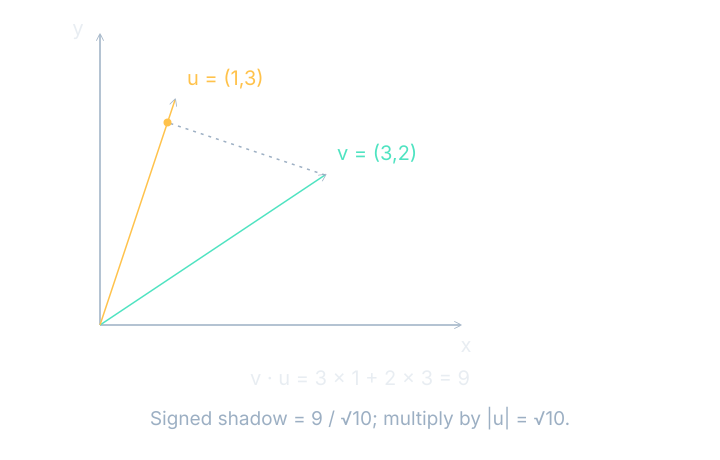
Project v perpendicularly onto the line containing u. The signed length of that shadow tells us how much of v points along u’s direction. The dot product equals that signed length multiplied by u’s length. It is therefore not a distance: doubling u doubles the dot product even if its direction stays exactly the same.

A similarity is a specified way of comparing how alike two inputs are. Dot products can serve that purpose, but their size reflects both direction and magnitude. If we want direction alone, we first divide each nonzero vector by its length. This division is called normalization. A zero vector has no direction to normalize.

The compact form uses i to visit corresponding entries in both vectors. The bold letters name whole vectors; the subscripts select their individual numbers. This is the same matching-and-adding operation that produced a row of our transformed point, now written without choosing a particular number of entries.

In words: multiply matching entries of the two vectors, then add the products.

A positive dot product indicates some alignment, zero indicates perpendicular directions for nonzero planar vectors, and a negative value indicates an opposing component. These statements describe a comparison, not the truth of a prediction. A model must still learn which transformations and comparisons help its particular task.

Area changes; translation needs an extra entry

The unit square lets us measure how much a transform expands or compresses space. Its determinant is the signed area factor. For a two-by-two matrix with rows (a,b) and (c,d), we calculate ad−bc. The magnitude gives the area factor; a negative sign records an orientation reversal. A zero determinant means the square’s area collapses.

Our stretch has determinant 2×1−0×0=2: twice the area. The flip has determinant −1×1−0×0=−1: unchanged area with reversed orientation. The collapse has determinant 1×0−1×0=0. These statements are about an entire small patch of the plane, not the distance one selected point traveled.

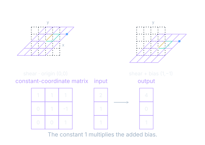
There is one movement those two-by-two matrices cannot perform: shifting the origin away from itself. Multiply any row by (0,0) and every product is zero. To move the origin, we add a bias, the same offset for every input. A linear map followed by a translation is an affine map.

We will usually keep the bias as its own vector, because that makes the stored parameters easier to inspect. The appended coordinate explains why the two descriptions agree. Let y name the final output, W the warp, x the original point, and b the shared translation.

In words: move the point with the matrix, then shift every result by the same bias vector.

Order changes the result

Composition means applying one transformation after another. It may look as if two movements should commute, meaning their order would not matter. We can test that belief with one point. Let A stretch the horizontal direction by two and let B shear the plane. Both operations preserve straight lines, yet they do different things to a slanted direction.

See it move

Start with the shear and bias off. Drag a column arrow, then inspect the corresponding two matrix entries. Type those entries directly and verify that the same picture results. Switch between the grid, the small center-square picture, and the 300-point teaching lattice. The original coordinates remain fixed; each redraw applies the new transform to those original points.

Turn on the bias controls and repeat the comparison. The second transformation now moves both the already-warped point and the earlier translation. This explains why a combined affine transformation has both a combined matrix and a combined bias. The live readout reports those quantities alongside the selected point, so the picture and arithmetic can be checked together.

Where this shows up when you train

Every learned matrix changes how a model arranges its inputs. The grid gives us a way to visualize that change without pretending the model stores literal arrows. It stores entries; our arrows reveal what those entries do. Two columns are enough to describe our two-coordinate example, while larger matrices extend the same row-by-row recipe to more coordinates.

When debugging a learned transform, check a unit input and inspect the corresponding column. Then check one mixed input such as (2,1). These small probes connect a weight table to observable behavior. They also reveal a transposed or reordered table much faster than staring at a large collection of entries.

Where we’re headed

A learned layer uses this warp, then a shift, then a bend. We will put its wiring diagram beside the matrix and compute it. Continue to the next chapter.