What shape does it eat?
A recurrent model passes information through a chain of states. What if each position could compare itself directly with earlier positions before choosing what to mix? We can build that operation from dot products and weighted averages. The model will learn the vectors used for those comparisons, alongside the rest of its weights.
A transformer combines attention with transformations applied separately at each position. Its vocabulary is the set of available tokens, and we use V for the number of tokens in that set. E6 uses the same synthetic-name corpus and split as E5-names. Each character ID selects an embedding row. position encoding adds information about where the token sits; E6 learns these position vectors and adds them to the token embeddings.
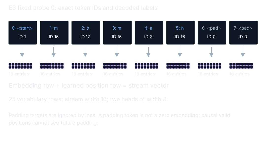
The recorded stream carries sixteen numbers per position. Its input has up to eight positions and its vocabulary has twenty-five tokens. The full parameter table contains 4,233 entries, including embeddings, position vectors, attention projections, normalization scales and biases, dense layers, and the output head. Right-padding targets are ignored by the loss. Padding is not the same thing as a zero embedding, and E6 does not apply a separate padding mask inside attention.
Each position chooses a mixture
A query is a vector used to score information to retrieve. A key is the vector compared with it to make a score. A value is the vector that will be mixed using the resulting shares. A head is one learned query, key, and value transformation with its own attention calculation. E6 has two heads, each using eight coordinates; our hand example uses two coordinates so we can check every product.
transpose swaps a matrix’s rows and columns without changing its entries. A matrix containing row-shaped keys is transposed so query rows can meet key columns in a matrix product. We divide each query-key dot product by the square root of the key width, then apply softmax across the allowed keys. The causal mask excludes keys later than the query. Excluded cells do not enter the denominator as small positive shares.
Compute all the scores and the mixture
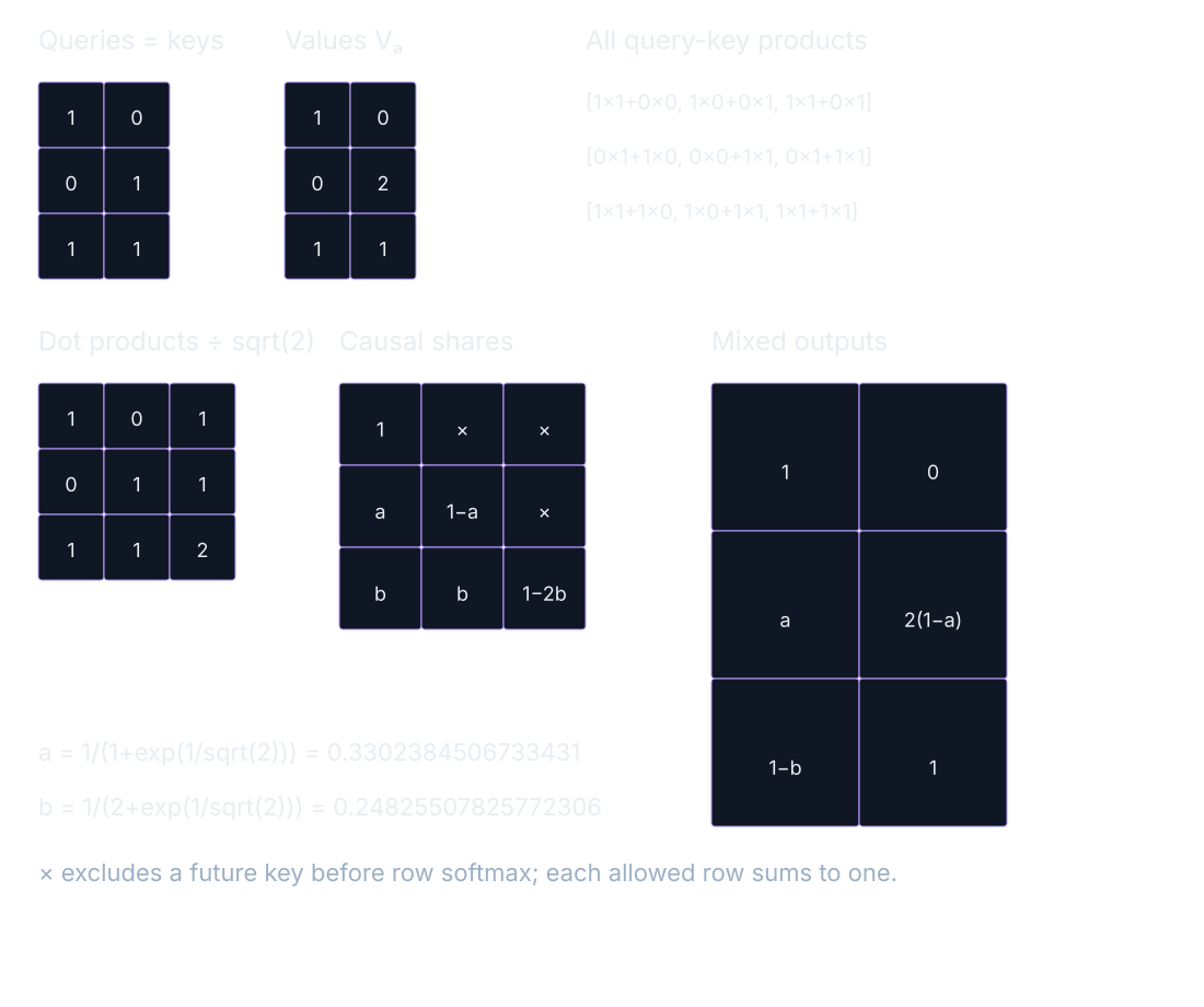
Our three query vectors and three key vectors are both (1,0), (0,1), (1,1). The value vectors are (1,0), (0,2), (1,1). We deliberately make the second value different from its key to keep their jobs distinct. A key determines a comparison score; a value supplies the information mixed after that comparison.
All nine comparisons
The first query gives [1×1+0×0,1×0+0×1,1×1+0×1]=[1,0,1]. The second gives [0×1+1×0,0×0+1×1,0×1+1×1]=[0,1,1]. The third gives [1×1+1×0,1×0+1×1,1×1+1×1]=[1,1,2]. Dividing by sqrt(2) gives rows [0.7071067811865475,0,0.7071067811865475], [0,0.7071067811865475,0.7071067811865475], and [0.7071067811865475,0.7071067811865475,1.414213562373095].
Exponentials and denominators
Exponentiating gives [2.028114981647472,1,2.028114981647472], [1,2.028114981647472,2.028114981647472], and [2.028114981647472,2.028114981647472,4.113250378782927]. Without masking, the row denominators are 5.056229963294944, 5.056229963294944, and 8.169480342077872. Divide every exponential by its row total. The shares are [0.4011120926797859,0.1977758146404282,0.4011120926797859], [0.1977758146404282,0.4011120926797859,0.4011120926797859], and [0.24825507825772306,0.24825507825772306,0.5034898434845538].
In words: exponentiate each scaled score and divide by the total for that query row. We have now computed every unmasked mixing share; the next operation changes which keys are allowed to contribute.
Remove future positions, then mix values
With masking, the denominators become 2.028114981647472, 3.028114981647472, and 8.169480342077872. The first row’s shares are [1,0,0], giving output (1,0). Let a=1/(1+exp(1/sqrt(2)))=0.3302384506733431. The second shares are (a,1−a,0), giving (a,2(1−a))=(0.3302384506733431,1.3395230986533138). Let b=1/(2+exp(1/sqrt(2)))=0.24825507825772306. The last shares are (b,b,1−2b), giving (1−b,1)=(0.7517449217422769,1).
For comparison, the unmasked output rows are (0.8022241853595719,0.7966637219606423), (0.5988879073202141,1.2033362780393577), and (0.7517449217422769,1). The last row stays unchanged because it has no future key to exclude. Bold Q and K collect queries and keys; bold V with subscript a collects attention values, distinct from vocabulary size V. The key width is d with subscript k, and bold M is the no-future mask:
$$\mathrm{Attention}(\mathbf{Q},\mathbf{K},\mathbf{V}_{\!a})=\mathrm{softmax}\!\left(\frac{\mathbf{Q}\mathbf{K}^{\top}}{\sqrt{d_k}}+\mathbf{M}\right)\mathbf{V}_{\!a}$$In words: score each query against the keys, scale the scores, apply the no-future mask, turn scores into shares, then mix the value vectors.
Read the actual attention during training
The trained attention arrays belong to fixed recorded token sequences. Their axes identify probe, head, query position, and key position. Selecting a different head changes which learned comparison we inspect. It does not mean we selected an independent model or a different validation split. Keep the token labels beside the grid so a bright cell refers to identifiable positions.
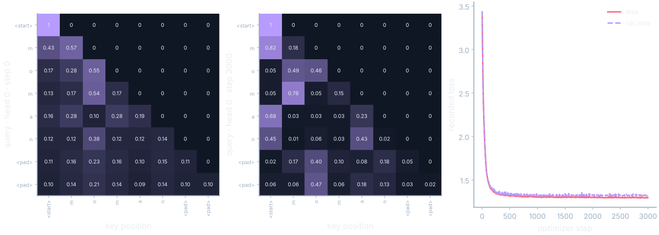
At step 3000, E6’s loss is 1.295941 and validation loss is 1.319666, from media/runs/E6.summary.json#/values/loss_at_3000 and /values/final_val_loss, both at series index 3000. E5-names finishes with validation loss 1.325217 at index 2000. The recorded losses are comparable on their shared task, but the differing update budgets and architectures prevent a broad conclusion about which family needs more data.
Where this shows up when you train
Attention is only one branch of E6’s computation. A residual adds a branch’s output to the incoming stream. In a hand example, stream (1,0) plus update (0,1) becomes (1,1). layer normalization centers and rescales one token vector, then applies learned scale and bias. E6 uses it before each branch. Its sixteen-coordinate stream keeps the same width across those additions.
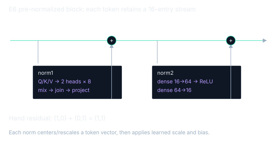
The first branch normalizes, calculates attention, joins the two heads, and projects their outputs before adding to the stream. The second normalizes, expands through a dense layer, applies ReLU, contracts back to stream width, and adds again. A final head produces vocabulary logits. The operations after attention can therefore change the eventual prediction even if the attention shares look similar.
Keep the query row fixed while editing one value coordinate; the shares stay fixed while the weighted output changes. This isolates the two roles with a direct numerical experiment.
What you now know
- Attention scores produce row-normalized mixing shares.
- Values carry the information combined by those shares.
- A trained head’s pattern does not by itself establish a causal explanation.
Where we’re headed
A graph network also mixes neighbors, but its connections come from an observed edge list. Continue the story.