Did It Actually Learn? Evaluation

What did the model beat?

The training process finished and printed a score. Did the model learn something useful, or did it perform a complicated version of an easy guess? We need a comparison rule, an evaluation population, and a definition of success before we can answer. The final loss line is evidence, but it is not a verdict by itself.

A majority-class baseline always predicts the most common training label. A mean baseline predicts the mean training target. A persistence baseline predicts the last observed value as the next one. We fit each comparison rule using training information and score it on the same evaluation examples as the model. A baseline tested on different data is not an equivalent opponent.

Reading the Graphs follows a weather model’s validation margin over an advection baseline across recorded epochs, showing how a “beat the baseline” checkpoint score can stall while loss keeps falling.

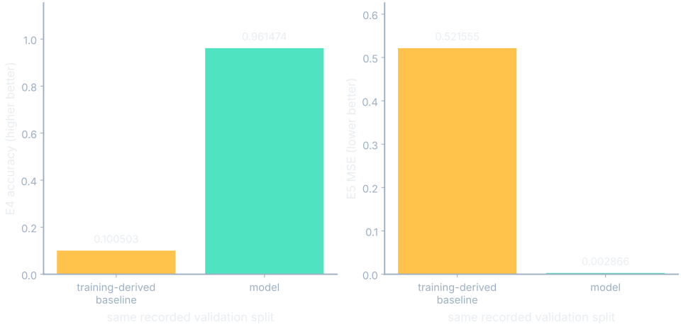
E4’s baseline and model are compared using validation classification accuracy, where higher is better. E5’s numerical model and its baseline are compared using mean squared error, where lower is better. The figure reads the actual baseline metadata beside the recorded final model metrics. We keep their axes separate because an accuracy fraction and a squared numerical error have different units and different meanings.

Count the kinds of error

MAE: Mean absolute error.

A confusion matrix records truth rows and prediction columns. For a binary task, “positive” names the event we choose to focus on. true positive means a positive prediction on an actual positive; false positive means a positive prediction on an actual negative. false negative means we missed an actual positive, and true negative means we correctly rejected an actual negative. The same event keeps the same definition across all four counts.

Our hand matrix is [[4,1],[2,3]], ordered negative then positive on both axes. Thus true negatives are four, false positives one, false negatives two, and true positives three. Accuracy is (4+3)/(4+1+2+3)=7/10. Precision asks what fraction of predicted positives were right. Recall asks what fraction of actual positives were found. Their denominators answer different questions even though both numerators count the same three true positives.

In the formulas, TP, FP, and FN stand for the counts just defined. N is the number of evaluated examples, y is the true numerical target, and y with a hat is the prediction. RMSE names root mean squared error. Write the counts or error values beside each formula so a score remains traceable to individual observations:

In words: precision asks what fraction of predicted positives were right; recall asks what fraction of actual positives were found.

In words: combine precision and recall through their harmonic mean, written here using counts.

In words: average squared misses, then take the square root to return to the target’s units.

Scores allow different decision rules

AUC: Area under a named curve, here the receiver operating characteristic.

A classifier gives scores or probabilities before we choose a decision rule. For one selected digit, we can call the case positive when that digit’s probability is at least a threshold. Lowering the threshold usually admits more positives and more false alarms; raising it usually rejects more of both. The threshold expresses a decision tradeoff, not a change to the model’s learned weights.

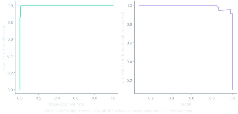
E4 records validation probabilities and labels at 31 confusion checkpoints: steps 0,100,…,3000. Each contains all 597 validation examples and ten class probabilities. The widget defaults to digit one as positive, with all other digits negative. It predicts positive when the exported probability is greater than or equal to the threshold. Equal rounded scores move together; the interface does not invent an ordering inside a tie.

Use the final assessment once

We can compute a per-class recall at every stored confusion checkpoint by dividing the diagonal count by that truth row’s total. This shows whether improvements are spread across classes or concentrated in a few. Choose the development checkpoint before opening the final test. Repeatedly selecting whichever checkpoint wins on that final set would turn it into another development set.

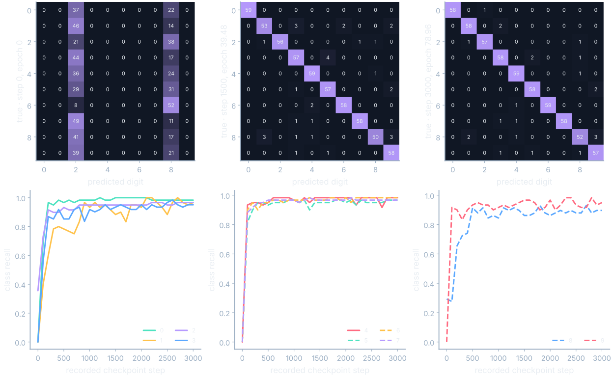
The matrices use their actual recorded steps and epochs, with the same color scale. The middle available checkpoint is not relabeled as an invented “epoch five.” Similarly, a metric calculated from checkpoint probabilities belongs to that checkpoint even while the optimizer cursor points between checkpoints. The step badge tells us where the evidence came from. An interface can hold a previous frame without pretending to have measured an intermediate evaluation.

distribution shift is a difference between development data and the inputs encountered later. A model selected on these digit images can encounter new stroke styles, image scales, or preprocessing upstream. A strong validation score measures the given split, not every later population. We cannot diagnose the exact source of an external failure from an accuracy drop alone; we must inspect both the changed inputs and the procedure that produced the original score.

Where this shows up when you train

Before evaluating a candidate, write the baseline, metric, split, positive class if relevant, and acceptance criterion. If missed events and false alarms have different costs, make that decision tradeoff explicit. A model’s probability threshold should serve the intended use rather than be tuned until one attractive scalar appears. Retain the confusion counts alongside the scalar so another reader can reconstruct how the criterion was applied.

Where we’re headed

We can evaluate success. Next we will use the measurements to diagnose what failed and check a repair. Continue the story.