Nowcasting the Radar

The problem

A radar loop shows rain moving now. What should we draw after the last observed frame? A nowcast is a short-range forecast. reflectivity (dBZ) describes the echo strength shown in these fields. We predict that quantity rather than claiming to predict every part of the weather.

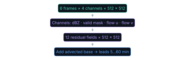
A lead time tells us how far ahead the prediction looks. The task asks for a field every 5 minutes through 60 minutes. A forecast is useful only in comparison with what a simpler method could already do from the same observations. Source §3.

The data

Each input frame contains reflectivity, a valid-data mask, and horizontal motion components. optical flow estimates that motion from the image sequence. advection carries the existing echoes forward. The advected field is an explicit base prediction, not a hidden target. Source §3.

The model never reads infrared imagery in this base run. Its input is recent radar and motion, with an advected base. The infrared-input idea belongs to a later experiment; it cannot be credited for this result. Source §3.

The base run uses 13,208 training and 441 validation sequences, with 34 held-out days. The split rules exclude shared days and nearby training anchors. Read the split chapter alongside those counts: many neighboring pixels do not create equally many independent weather situations. Source §3.

The model

The architecture combines local convolutional features with a carried recurrent state. A ConvGRU updates a grid of remembered features as frames arrive. The model therefore retains local spatial relationships while combining information over time. A U-Net gathers context at coarser scales, then combines it with finer features while decoding the output.

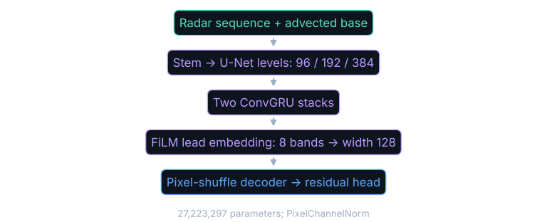
FiLM scales and shifts features according to the requested lead. Here the lead embedding uses 8 sinusoidal bands and width 128. The full model has 27,223,297 parameters; the recurrent stacks account for 77 percent. The output is a residual added to the advected base, allowing the network to change that forecast rather than starting from an empty field. Source §3.

Where this comes from

The architecture is not novel: our convolutional recurrence follows Shi et al.’s ConvLSTM (2015) and TrajGRU (2017). We compare with advection and S-PROG in Pulkkinen et al.’s pySTEPS (2019). DGMR (Ravuri et al., 2021), the MetNet family, and NowcastNet (Zhang et al., 2023) are state-of-the-art references we do not claim to match. MetNet-1 (2020) and MetNet-3 (2023) are arXiv preprints; MetNet-2 (2022) is peer-reviewed. Ours is the corpus, regional fine-tunes, day-block splits, and rigor pass. Source §6.

The loss and why that loss

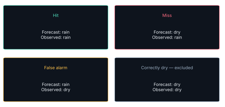
critical success index (CSI) measures event overlap using the boxes above. Correctly dry pixels do not enter the denominator.

In words: divide correct event predictions by all pixels where either the prediction or the observation says an event occurred.

In words: combine intensity-weighted absolute error over valid pixels and several scales with a differentiable event-score penalty.

The soft event boundary uses a 2 dBZ sigmoid at thresholds of 20 and 35 dBZ. A 63.75 dBZ core counts five times as much as a clear pixel in the intensity weighting. The point is to make meaningful echoes matter to the update, not to claim that the proxy loss and the final task score are interchangeable. Source §3.

Training as it actually ran

The run record gives batch size 8, distributed training on 2 GPUs, a base learning rate of 2e-4 with the head five times faster, and 8 epochs. Its duration summaries are 10.87 hours and 78.5 minutes per epoch. Those are the reported run descriptors; the copied telemetry is retained separately so differences in logging scope remain inspectable. Source §3.

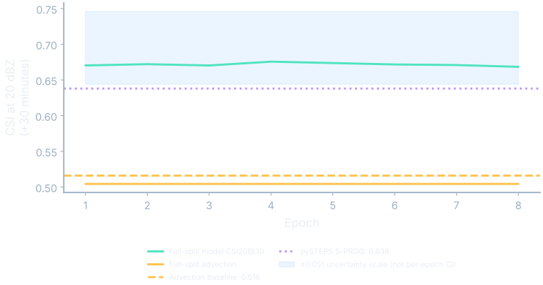
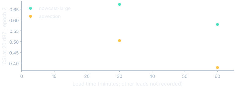
The quality-review result is CSI20@30 of 0.695 versus S-PROG at 0.638, with the model interval [0.648, 0.737]. This re-score uses a day-stratified subset of 24 of the 441 samples across 17 days. The same checkpoint scores 0.672 against full-split in-house advection 0.504; a full-split S-PROG value is unavailable here. Its saved-best selection is epoch 2; epoch 4 has the highest logged CSI20. In-house advection at 0.516 is the weaker comparison; stock Lucas–Kanade extrapolation improves that lane by about 0.09 CSI, so S-PROG is the baseline to headline. Source §3.

Outputs

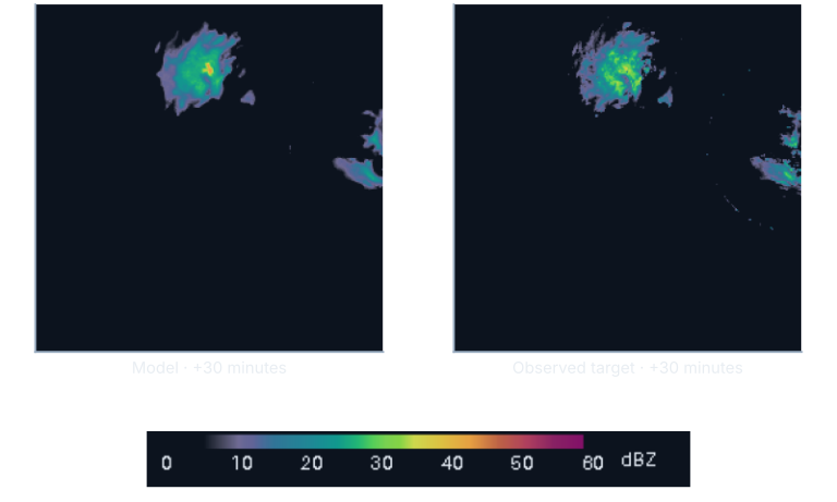
The strip compares a saved forecast and its target at the same valid time. The regional fine-tune is distinct from the base model evaluation. It cannot show a visual advection comparison because that field was not saved.

See it move: the epoch flipbook uses retained v2 probes and their matching epoch scores. The lead scrubber changes the requested forecast horizon instead. Those are different axes: later training is not later weather. The supplied v2 images show the middle lead only, while its score table retains the middle and final leads.

What it is not

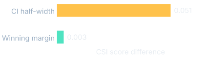
A confidence interval expresses uncertainty in an estimate. The day-block procedure respects shared weather within a day. The winning margin was much smaller than the uncertainty scale, so choosing the peak epoch does not establish a reliable advantage over its neighbors. The rigor pass exists to test that uncertainty. Its warm-start sequence is described as flat; small changes inside the day-block uncertainty do not establish improvement. Source §3.

Before comparing two forecast images, check their starting time and requested lead. A later observation can look like a better forecast merely because it has seen more of the event. Likewise, changing a reflectivity threshold changes which pixels count as events, so the threshold belongs in both the score label and the comparison protocol.

Where this shows up when you train

Choose a stopping rule that measures the behavior you need. Look at event frequency as well as overlap. Keep the review baseline, retained epoch metrics, region, and forecast lead visible; otherwise a convincing curve can quietly answer a different question.

Run this yourself

trainkit nowcast samples/blobs.npz --output nowcast-output

The command writes run.json and model.json. Add --dry-run to preview the replacement targets. Keep your output separate from the bundled book artifacts. The run records the data shapes, split, objective, baseline, model score, and elapsed time; the model export contains the actual learned weights.

Repeat the run before changing the recipe. Then change a single input or model choice and compare on the same held-out examples. A different random split can change a score even when the learning rule is unchanged. Keeping the original baseline makes it possible to distinguish an improvement in the learner from an easier evaluation problem.

Where we’re headed

Next we will carry the same questions into Doppler Everywhere (designed, not yet trained).