Which answer has to wait?
Why do training jobs often use a graphics processor? The answer starts inside a dot product, before we discuss any hardware. We already know the layer’s weights and inputs. If we draw which answers depend on which earlier answers, we can see which calculations can run together and which must wait.
Use our output matrix [[1,−1,0],[0,1,1]] on input (1,1,0). The two output sums are 0 and 1. Output one does not need output two’s answer, and output two does not need output one’s. That makes the outputs parallel work: independent calculations can proceed concurrently when hardware resources are available.
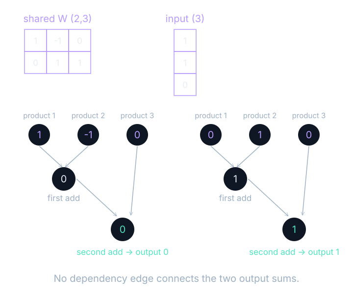
A data dependency occurs when a calculation needs a result from an earlier calculation. Each output sum still depends on its products. We can calculate the products independently, then combine them. The independence between output cells does not erase the need to combine terms inside each dot product. This distinction prevents an appealing but incorrect story in which every multiply-add is independent of every other operation.
Imagine marking one output cell and tracing only its incoming edges. Its three products belong to that output’s calculation. Mark a second output and trace its incoming edges: the input data are shared, but the accumulated result is separate. Shared inputs are compatible with independent outputs as long as those inputs remain available and unchanged during the calculation.
Count the arithmetic before timing it
Two outputs and three inputs require 2×3=6 products and 2×(3−1)=4 additions before bias. A FLOP is one floating-point arithmetic operation. A multiply-add is commonly counted as two FLOPs. For batch size B, a useful approximate layer count is 2×n_out×n_in×B. It is an operation count, not a number of seconds.
The approximation treats each output contribution as a multiply-add. The exact addition count differs because the first product need not be added to a previous term, and a bias adds another operation. For large products those differences are small relative to the total, but stating the convention matters when we compare rates. The hardware may also execute an instruction that combines multiplication and addition while the FLOP count still assigns it two operations.
Some work remains a chain
Some computations present a very different dependency picture. Consider a loop that maintains a running total. It starts from zero, reads an entry, updates its state, then reads the next entry. Each literal loop iteration needs the state produced by the previous iteration. Adding hardware lanes does not remove that edge from the program.
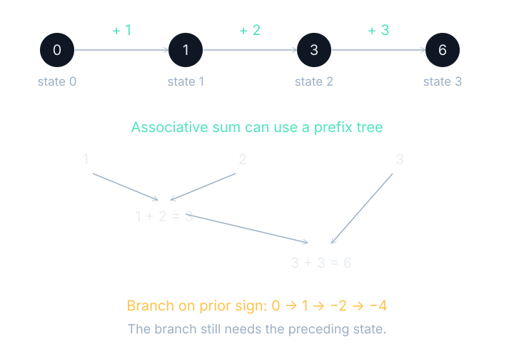
For entries [1,2,3], the states are 0→1→3→6. The third state uses the second state. Addition has a useful property: we can group terms differently while preserving the exact-arithmetic sum. A parallel prefix algorithm exploits this to compute all partial sums with a different graph. Floating-point regrouping may change small rounding details, so equivalence needs a stated tolerance.
A branch that depends on the previous state can prevent the same rearrangement. For example, if the sign of the accumulated value decides whether to add or subtract the next input, the later choice is not known until that earlier state is known. Before declaring a loop parallel, inspect the mathematical dependency as well as the code’s visible loop syntax.
Latency measures elapsed time to finish one operation. Throughput measures how much work finishes per unit time. A processor can have high throughput while taking longer to finish a tiny individual request, especially when setup is involved. A kernel is a device program launched across many work items. Launching it has a cost even if the arithmetic inside is short.
Memory bandwidth measures bytes moved per unit time. VRAM means video random-access memory, the storage on a graphics device. Inputs must be available where the calculation executes. If they start in CPU memory, copying them to the device may dominate a small calculation. If a training loop keeps data and parameters on the device, later operations can reuse them there.
Read the measurement, including copying
We can now read an actual benchmark without asking it to answer more than it measured. B1 records matrix-vector products and square matrix products at a sequence of sizes. It does not measure a fixed neural-network batch of sixty-four examples, and it does not measure a complete training epoch. Its horizontal axis is the side length of a square matrix.
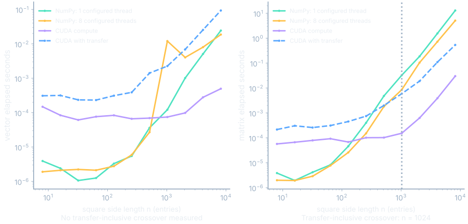
Each panel shows four recorded timing modes: NumPy with one configured thread, NumPy with eight configured threads, CUDA compute, and CUDA with transfers. Both NumPy modes were restricted to four CPU cores. CUDA is the programming platform used for these graphics-device measurements. Its compute timing and transfer-inclusive timing answer different questions about where the operation begins and ends.
The transfer-inclusive square matrix product first beats both measured CPU modes at size 1024. No tested matrix-vector size beats both CPU modes after transfer. The recorded vector crossover is null: no crossover was found among the tested sizes. Null does not mean zero seconds, and it does not identify some untested threshold.
The axes are logarithmic so both small and large sizes remain visible. Equal spacing represents equal multiplicative ratios, not equal additions. A point that breaks an otherwise smooth-looking trend remains part of the measured record. We retain it rather than drawing a tidier curve and promising a speedup that the recording did not establish.
The source is B1.json’s series, with the crossover summaries in B1.summary.json. Those results belong to the recorded shape, dtype, hardware, thread configuration, and timing boundary. The figure is evidence for those settings. It is not a universal law that any operation exceeding 1024 entries should move to a graphics processor.
Change the amount of independent work
The simulator below separates scheduling from measured elapsed time. Begin with one lane and the fixed two-by-three layer. Step through the products and each output’s additions. Then provide a second lane and watch the two output reductions advance independently. The drawing explains a dependency advantage without claiming to emulate CUDA’s actual execution machinery.
See it move
Change the batch size while preserving the shared weight table. More examples create more independent output cells, each with its own reduction. Increase the lane count and observe when additional lanes stop helping the current small workload. If there are fewer independent jobs than lanes, some lanes have no useful work to do.
Open the measured pane separately and select one of B1’s recorded square sizes. Those values are seconds; the scheduler’s values are teaching ticks. A rectangular layer with an added bias has no exact B1 match. Keeping that distinction visible lets us use a simple model to explain behavior without manufacturing a benchmark result.
Where this shows up when you train
A training program often benefits from keeping weights, intermediate values, and batches on the device across many operations. That spreads initial transfer costs over more useful work. It still needs to feed the device, respect dependencies between layers, and avoid materializing unnecessary arrays. Independent arithmetic is one condition for good performance, not a complete performance diagnosis.
The next step is to change how we express work. Some programs hide independent calculations inside a serial-looking loop. We will take three small examples, preserve their checkable arithmetic, and expose their array structure so a numerical library can schedule the work more effectively.
What you now know
- Independent outputs can be computed concurrently.
- Transfers and launch overhead can dominate small operations.
- A measured crossover belongs to a specified operation and machine.
Where we’re headed
We can now look inside an ordinary loop and separate the mathematical dependencies from the order the program imposed. Continue to the next chapter.