True Colour from Three Bands

The problem

Why does a satellite picture need a learned color recipe at all? A display needs a red, green, and blue value at each location. Our input stack supplies red and blue reflectance plus a near-infrared vegetation band. We will follow one mapping from measured bands to a visible picture, using the dense layers and held-out evaluation we already know.

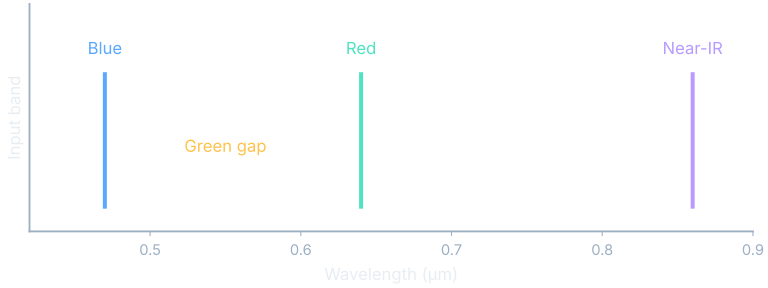
true colour means a rendering intended to resemble human color vision. synthetic green supplies the missing display value from other bands. A fixed recipe always applies its prescribed calculation; a learned recipe adjusts its weights against reference images. The useful question is whether those adjustments improve an unseen day, rather than whether a picture looks more vivid.

The data

A coincident pair matches the geostationary input with a nearby polar-satellite observation. The targets are corrected-reflectance true-color products from NASA GIBS. We need the match because a moving cloud can make a correct color prediction disagree with a reference that saw different weather. Source §1.

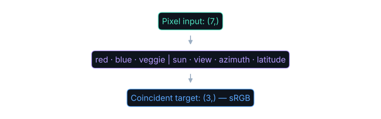
The input contains red, blue, and veggie reflectance, sun zenith, view zenith, relative azimuth, and latitude. Its fixed normalization divisors are [1.5, 1.5, 1.5, 90, 90, 180, 90]. Output values lie in [0, 1]. Geometry matters because illumination and viewing conditions change how a surface appears. Source §1.

The model

The model applies the same dense network independently at every pixel. That is a strong architectural restriction: it can respond to the feature list, but it cannot inspect a neighboring coastline or cloud edge. Follow the arrows as array operations, using the dense-network chapter for the underlying weighted sums.

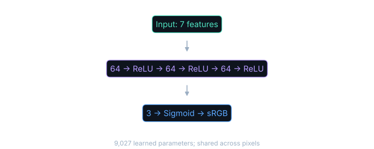
A hidden activation changes which combinations can influence the next layer. The final squash keeps the display values within the allowed range. Neither operation supplies spatial context. Feeding the same feature list at another location gives the same output; any location-specific difference must arrive through an input feature. We should therefore judge this network as a color mapper, rather than a general image-restoration system.

Where this comes from

The architecture is not novel: shared dense layers provide the learned mapping. Synthetic green follows CIMSS/NOAA’s recipe described by Bah et al. (2018) and JMA’s color reproduction in Murata et al. (2018); Broomhall et al. (2019) address vivid-color correction. We found essentially one precedent for learned reconstruction compared with a polar-orbiter reference: Gonzalez and Yamamoto (2020), validated against MODIS. Ours is the matched corpus and per-pixel correction fitted against those reference colors, not an invention of synthetic green. Source §6.

The loss and why that loss

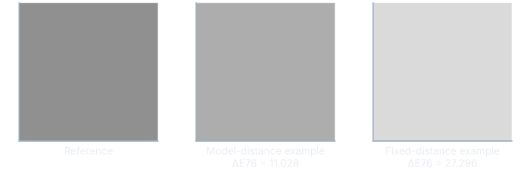
CIE Lab places colors in coordinates where distance roughly follows visible difference. ΔE is read “delta E”; here ΔE76 is the straight-line Lab distance. For coordinate differences dL, da, and db, $\Delta E76=\sqrt{dL^2+da^2+db^2}$: zero means identical colors, and distance has no universal upper bound. Roughly one unit is a barely visible reference, not a universal perceptual threshold. The model’s 11.028 versus the fixed formula’s 27.296 means about eleven rather than twenty-seven Lab units from the reference on average. Neither is a count of incorrect pixels. No confidence interval was measured: the observed gap is large, but its reliability across new days is unquantified. The older distance formula over-weights saturated colors; we also inspect matched scenes and error maps. Source §1.

In words: convert the predicted color, y-hat, and target color, y, to Lab, square their coordinate differences, and average them.

This is the error measure from How Wrong Is It? with a color conversion in front. Differentiability lets the gradient pass through that conversion to the network. The loss rewards agreement with the matched reference; it does not directly reward dramatic saturation or a reader’s preferred aesthetic. Source §1.

Training as it actually ran

The Himawari run used batches of 8,192 pixels, Adam with a constant learning rate of 0.001, and 30 epochs. The run summary reports 0.31 hours overall and 0.2 minutes per epoch. Those separately reported timing summaries are retained as reported, not used to derive each other. The host has two RTX 4080 cards; that inventory alone does not mean this pixel model used both. Source §1.

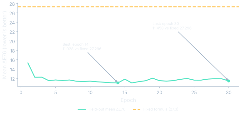
The best held-out mean error is 11.028 at epoch 14, against 27.296 for the fixed formula on the same pixels. The final epoch, 30, is slightly worse at 11.458 versus the same fixed-formula 27.296. The fixed schedule had no early stopping, so we keep the earlier checkpoint rather than calling the final state the best. This establishes an aggregate improvement, not improvement at every pixel. A difficult surface can still become worse while the mean improves. Source §1.

Outputs

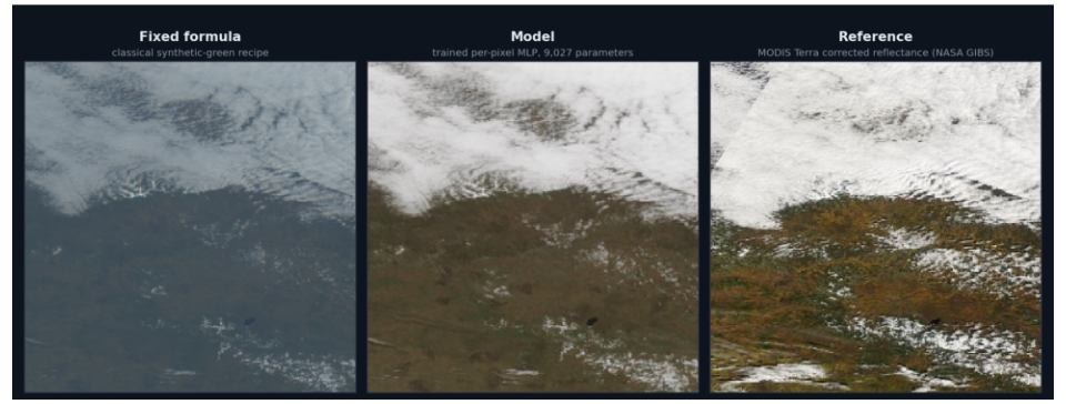
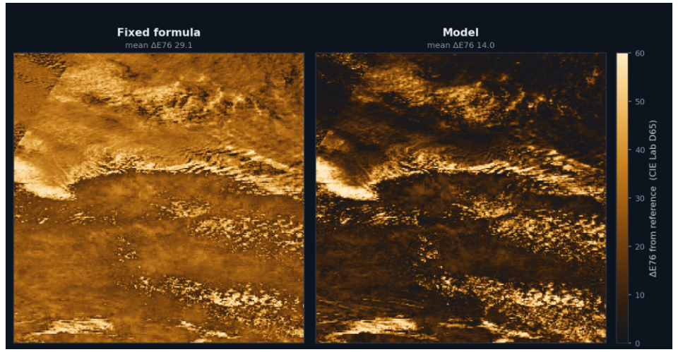
This comparison restores the original spatial planes, so neighboring pixels really are geographic neighbors. The reference resolves finer detail than Himawari; edge differences include sensor resolution and alignment. This scene’s model mean is 13.98 against fixed 29.09, distinct from run-wide 11.028 against 27.296. Neither comparison has a day-block confidence interval. Source §7.

See it move: keep a probe identity fixed and scrub the epochs. The score below the image belongs to the whole held-out evaluation, not just the pixels visible in that probe. The training probe is a shuffled pixel atlas, distinct from the spatial scene above. A stable input identity makes changes across checkpoints interpretable.

The color mixer is a browser surrogate fitted to copied model predictions. It omits geometry and is deliberately much smaller than the production network. Its fixed swatch evaluates the production formula at the slider inputs with sun angle held constant. Treat the interaction as a demonstration of a learned mapping, not as production satellite processing.

What it is not

Training sun zenith spans 12°–79°, with a cap at 85°. We have no license to extend this daytime result into night. The run supplies no confidence interval for this particular color comparison; the absence of an interval is not evidence that the mean is exact across other days. Source §1.

Where this shows up when you train

Separate the task you optimized from the task a reader might assume. A successful color mapper is a useful result on its own. Calling it a scene corrector would hide the most important limitation of its input representation. Keep the split, baseline, and pixel-selection rule beside the headline.

Run this yourself

trainkit colour samples/colour.csv --output colour-output

The command writes run.json and model.json. Add --dry-run to preview the replacement targets. Keep your output separate from the bundled book artifacts. The run records the data shapes, split, objective, baseline, model score, and elapsed time; the model export contains the actual learned weights.

Repeat the run before changing the recipe. Then change a single input or model choice and compare on the same held-out examples. A different random split can change a score even when the learning rule is unchanged. Keeping the original baseline makes it possible to distinguish an improvement in the learner from an easier evaluation problem.

Where we’re headed

Next we will carry the same questions into the super-resolution chapter.