The problem
A radar map can be blank because no radar reaches that place, rather than because the sky is clear. This chapter describes a proposed way to fill that observation gap from satellites. satellite-derived is the essential label: the planned product estimates reflectivity. Its title does not make it a measurement of Doppler velocity.
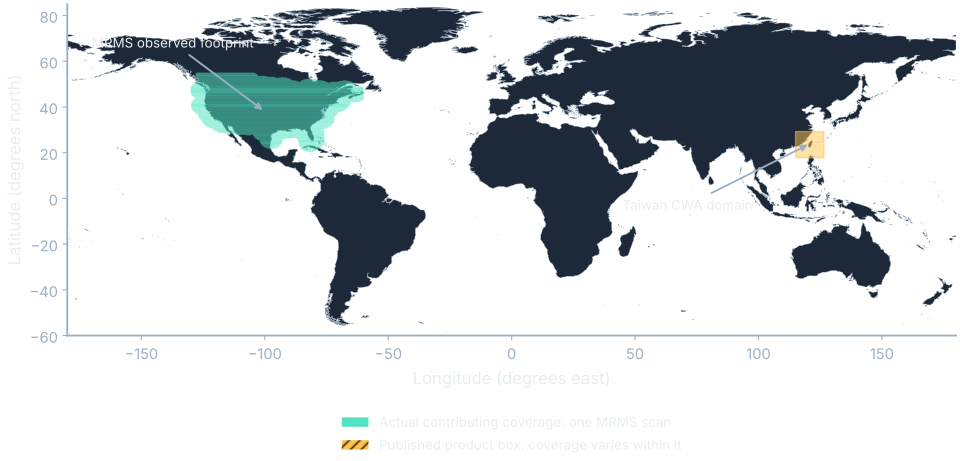
The design separates Observed from Satellite in the interface. That distinction should travel with the image wherever it is displayed. The proposed global product has a 10-minute cadence at approximately 4 km, but no trained model or model output exists yet. These are design choices, not measured product performance. Source §4.
The data
An infrared image measures radiation associated with the cloud top. brightness temperature describes that radiance on a temperature scale. It is useful information, but it is not a direct measurement of precipitation beneath the cloud. The same apparent cloud top can accompany different conditions lower in the atmosphere.
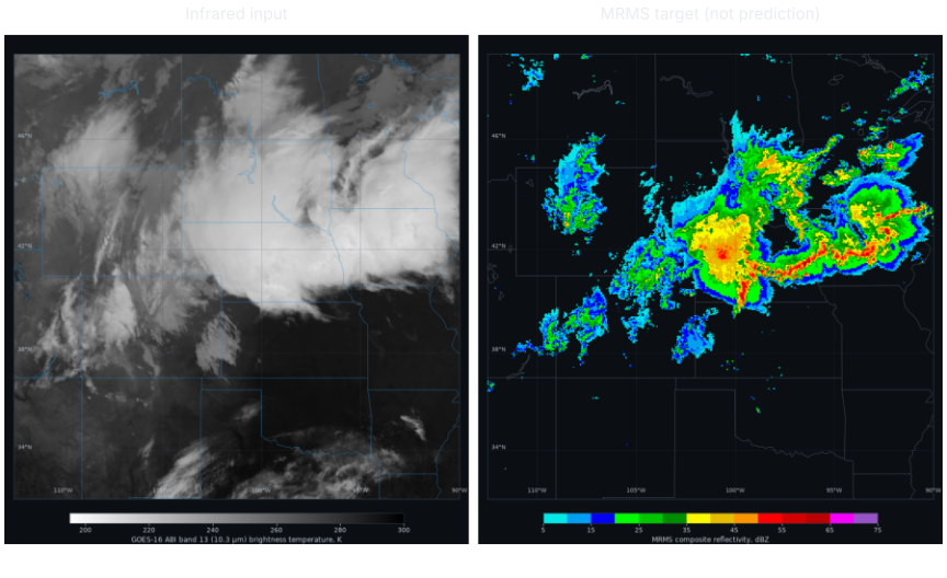
The proposed targets come from radar composites where radar exists: MRMS in CONUS, OPERA in Europe, AURA in Australia, IDEAM in Colombia, REDEMET in Brazil, and Taiwan CWA. A paired training example must align the satellite input and radar observation in space and time. A coincident target teaches a mapping; an unrelated attractive image does not. Source §4.
The model
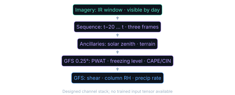
The design uses three frames from t−20 through t, visible imagery by day, and ancillary solar-zenith and terrain information. GFS fields arrive on a 0.25° grid and include atmospheric water, freezing level, instability and inhibition, wind shear, column humidity, and model precipitation rate. These names describe distinct physical clues; they do not imply that all inputs have already been collocated into a trained tensor. Source §4.
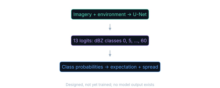
pipeline/src/metoc_pipeline/nowcast/model_large.py (NowcastUNetGRU). The distribution head is proposed, not implemented; design and class count: source §4.A U-Net combines local image features with broader context and returns an output at each pixel. The proposed size is approximately 10–25 million parameters, using the nowcast encoder’s general shape. It predicts class scores rather than one unconstrained scalar. Day and night variants and forecast heads at +30/+60 minutes are part of the design, not implemented performance claims. Source §4.
An ambiguous input should be able to say that rain is uncertain. Averaging incompatible target values with squared error can produce the “gray soup” described in the design: a middling value that matches neither a clear sky nor a strong echo. Assigning probability to classes makes the no-rain possibility explicit, while still allowing probability to be shared across rain strengths. Source §4.
Where this comes from
The architecture is not novel. Infrared-to-rain learning goes back to Hsu et al.’s PERSIANN (1997). Much closer is Hilburn, Ebert-Uphoff, and Miller’s GREMLIN (2021): satellite temperatures plus lightning mapped to MRMS reflectivity. Lee and Hilburn (2024) document its winter cold-surface failure. We are following this recent line with a planned multi-region corpus, environmental inputs, and explicit Observed/Satellite labeling. Ours is the planned cross-network corpus, the mask, and the forecast heads; no trained result yet establishes their value. Source §6.
The loss and why that loss
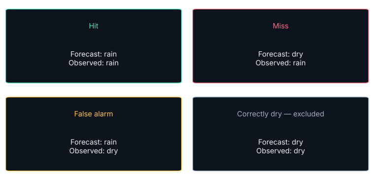
For the CSI event score, $\mathrm{CSI}=\mathrm{hits}/(\mathrm{hits}+\mathrm{misses}+\mathrm{false\ alarms})$, from zero (no overlap) to one (perfect overlap). The separate classroom toy scores 0.9988003969 versus its climatology baseline 0.2034505159: almost every toy event pixel agrees, compared with about one fifth for the reference. There is no production score or confidence band, and the toy has no repeated-run interval; neither proves the proposed system works. CSI ignores how severe a miss is, so the design also checks the stronger reflectivity threshold. Source §6.
$$L=-w_y\ln p(y\mid\mathbf{x})+L_{\text{CSI-aligned}}$$In words: penalize low probability on the observed class, multiply by that class’s weight, and add the planned event-score penalty.
Here x is the input feature collection, y is the observed class, p is its predicted probability, and w is the class weight. Cross-entropy gives a gradient even when the final display would round several different distributions to a similar shade. The additional CSI-aligned term focuses attention on the event thresholds used for evaluation. Source §4.
As in the loss chapter, the choice of objective encodes a priority. It does not prove the priority was achieved. We still need held-out predictions to find whether weighting increases useful detections or merely increases false alarms.
Training as it actually ran
No trained model exists. No epoch curve, learning rate, batch size, training duration, or held-out model score can be reported for this design. Corpus assembly is underway. An empty result is the accurate result for this section. Source §4.
The proposed gate evaluates held-out-region CSI at 20 and 35 dBZ against climatology, and repeats the comparison without the GFS environment block. Withholding regions asks whether the mapping travels beyond locations that supplied training radar. Removing an input group asks what that group contributes under a controlled comparison. Source §4.
We have no result for that gate yet. The planned comparison is useful because it tells us what evidence would change the chapter’s status. A model diagram, an assembled corpus, and a plausible objective are preparation for a measurement. None is a substitute for the measurement itself.
Outputs
The input/target pair is observed weather. The widgets use a separately trained synthetic classroom model: clicking an infrared location selects a toy cell, not a satellite-radar prediction.
See it move: shift the selected toy cell and watch the probability bars. The classroom model has broad synthetic categories, which the display distributes across the finer proposed reflectivity bins. That redistribution illustrates a chart format; it is not a learned probability distribution over production dBZ classes. The infrared frame is context for the intended interface only.
A wide distribution is not an automatically calibrated confidence statement. A model can also become confidently wrong outside its training conditions. The proposed region holdout matters here because the very places needing satellite-derived estimates may have different terrain, cloud regimes, or observing geometry from the radar-covered training sources.
What it is not
Climatology is the comparison named in the design: the usual frequency or pattern of the event provides a reference that does not depend on the current satellite image in the same way. A useful learned product must improve on that reference on the held-out region. Removing the environment inputs then tests whether the extra complexity earns its place. Source §4.
Where this shows up when you train
Distinguish the next experiment from a finished result. Here the honest headline is a question with a defined baseline and a proposed test. A reader should be able to tell what has been measured without inspecting the implementation or guessing from the polish of the diagram.
Before publishing a satellite-derived image, we would also need to establish what happens when an input is missing. A daytime visible channel cannot silently become a valid nighttime observation. The proposed day and night variants acknowledge that the available information changes. Their existence in a design does not prove a fallback has been trained or validated; the interface must keep the observation source and model status understandable to the person reading the map.
Worked example
For an illustrative three-class probability vector (0.5, 0.3, 0.2), suppose the first class is observed and its weight is 1. Its cross-entropy term is $-1\cdot\ln(0.5)=\ln(2)\approx 0.693$. Assigning that class probability 1 instead gives $-\ln(1)=0$. The loss rewards probability on the observed class, not the tallest-looking bar. Source §7.
Run this yourself
trainkit rainmap samples/ir-rain.npz --output rainmap-outputThe command writes run.json and model.json. Add --dry-run to preview the replacement targets. Keep your output separate from the bundled book artifacts. The run records the data shapes, split, objective, baseline, model score, and elapsed time; the model export contains the actual learned weights.
Worked example
The synthetic rain-or-heavy CSI result is 0.9988003969, compared with baseline 0.2034505159. Recorded training time is 7.192842874 seconds. Source §6.; media/runs/E13.summary.json#/values.
The toy gain is $0.9988003969-0.2034505159\approx 0.795$. It grades the union of rain and heavy-rain toy classes, not a production reflectivity threshold. No repeated-run interval was measured, so this is a measured example, not a significance claim. Source §6.
Repeat the run before changing the recipe. Then change a single input or model choice and compare on the same held-out examples. A different random split can change a score even when the learning rule is unchanged. Keeping the original baseline makes it possible to distinguish an improvement in the learner from an easier evaluation problem.
What you now know
- Satellite-derived reflectivity is an estimate, not an observed radar return or Doppler velocity.
- A distribution can express competing rain possibilities that one average hides.
- The architecture follows published work, but this production model has not been trained.
- The next evidence must come from held-out regions and an input ablation; the classroom toy cannot supply it.
Where we’re headed
We have reached the boundary between measured results and the next experiment. Return to Designing the Run to turn a proposed model into an inspectable test.