Name the symptom before its cause
noise floor: Variation or irreducible error below which a change is not distinguishable with the current measurement.
A loss curve looks wrong. The tempting response is to change several settings until it looks better. Let’s slow that decision down just enough to make the next run informative: name the symptom, state a hypothesis, choose one check, and decide what result would reject that hypothesis. A failed run can teach us something if we preserve what actually happened.
The evidence should include raw curves, the split, settings, and recorded status. Smoothing can hide a spike, while a finite loss can remain very high. “Diverged” sometimes describes poor learning informally, but nonfinite arithmetic is a more specific claim. We should not call a value NaN merely because it increased. The saved status and numeric entries let us distinguish those cases.
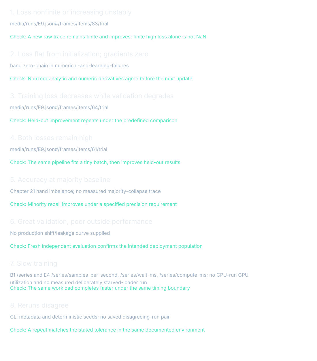
The eight cases cover numerical instability, zero gradients, a widening development gap, weak learning, majority-class behavior, outside-data failure, slow training, and disagreeing reruns. Some have actual E9 traces. Others are hand calculations or hypotheses without a recorded production example. Their evidence labels appear before the suggested answer so we do not confuse a useful diagnostic idea with an incident that was actually measured.
When arithmetic or learning stalls
A flat loss can mean that weights are not moving, that they are moving too little to matter, or that the chosen metric barely responds to their changes. Gradients help distinguish these possibilities. Check the actual parameter values as well as the plotted line. If a gradient is zero, ask which local factors produced it before treating zero as proof that the model reached a useful minimum.
A zero product path
Let the hand prediction be w₁w₂x, with input x=1, target 1, and both weights zero. The prediction is 0 and squared error is 1. The derivative with respect to w₁ contains w₂, and the derivative with respect to w₂ contains w₁. Both are therefore zero. A coordinate-wise finite difference also returns zero at this point. Moving both weights together can lower the loss, so this zero-initialized saddle is not a useful solution.
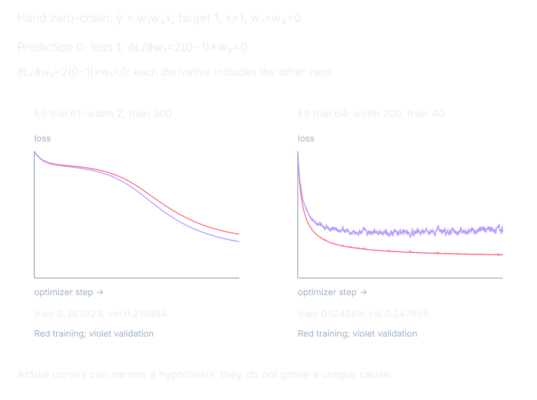
Changing the initialization can break that confirmed zero product path. First verify that the resulting analytic gradients agree with numerical differences; then take an update. A changed initialization alone is not an accepted repair if the subsequent loss and held-out checks still fail. This hand model is not a verified explanation of an external nowcast incident. It supplies a small counterexample to the assumption that zero gradient must mean the job is done.
When a good-looking score is misleading
A model near majority-class accuracy might be predicting only the common class, or it might be making a different mixture of mistakes. The aggregate accuracy cannot distinguish those possibilities. Read per-class confusion counts and label mappings first. Our explicit evidence is the hand example from evaluation: nine negatives, one positive, all-negative predictions, accuracy 9/10 and positive recall zero. No saved E9 per-class trace establishes a measured majority-collapse episode.
Excellent validation followed by poor external performance can arise from leakage or distribution shift. These causes require different investigations, and a single curve cannot separate them. Audit duplicate groups, temporal boundaries, and where preprocessing was fitted. Compare external inputs to the development population. A new independent evaluation can test the intended use, but repeatedly tuning against that evaluation turns it into development evidence too.
When it is slow or hard to reproduce
loader-bound: Execution limited by supplying input data rather than computing on it.
Slow training needs a timing boundary. Are we timing only an arithmetic kernel, a complete update, full validation, input loading, or exported diagnostic frames? Those are different workloads. E4’s recorded CPU run includes instrumentation. Its wait and compute fields give useful measurements, but their names alone do not tell us that a disk loader or GPU was idle.
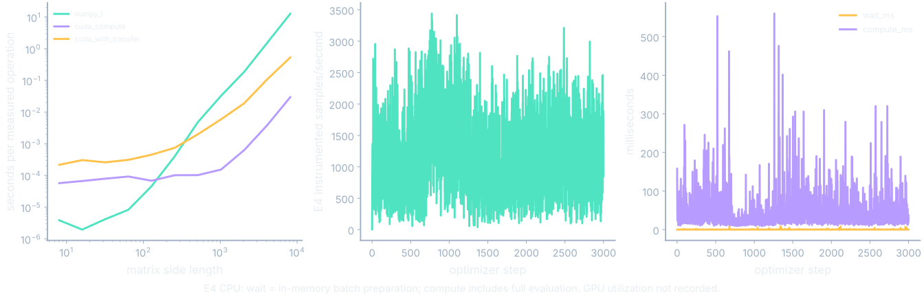
E4’s wait_ms measures in-memory batch preparation, including index selection, shuffle, and slicing. Its compute_ms measures update plus full-split evaluation, excluding the batch wait and frame export. GPU utilization is not recorded for this CPU run. B1 separately measures matrix compute and transfer-inclusive timings. We can compare those available intervals while keeping disk-loader starvation and GPU idling labeled as unmeasured hypotheses.
When reruns disagree, compare inputs and procedure before comparing only final accuracy. The data file, split indices, preprocessing, seed, parameter initialization, software version, and numerical operations can all matter. A seed does not promise identical results across platforms. A small early difference can later change the path of optimization, so the first differing state is often more informative than the size of the final gap.
Where this shows up when you train
Choose a case and describe the raw evidence before revealing a cause. Select a check that could disprove the proposed explanation. For the zero-chain example, nonzero checked derivatives after an initialization change support the immediate mechanism. For an overfitting hypothesis, a repeated held-out improvement under the predefined comparison is more relevant than a prettier training curve. Different symptoms require different acceptance evidence.
What you now know
- A symptom does not uniquely identify its cause.
- A repair needs a named check on appropriate data.
- Missing telemetry remains missing evidence.
Where we’re headed
We will now run the shipped tools, open their outputs and explain the numbers in our own model. Continue the story.