How Wrong Is It: Loss, Entropy, Cross-Entropy

Choose a ruler for the prediction

The model assigned class 1 a probability of about 0.682. If class 1 is the supplied answer, how wrong is that prediction? We need a ruler that scores more than whether the winning label matched. Different tasks need different rulers, so we will construct two and calculate their answers before using either to train.

A label is the supplied answer for an example. A loss is a scalar score comparing a prediction with its target. An objective is the quantity a training procedure tries to reduce. The loss makes a many-entry prediction comparable through one number, but that number only has meaning once we state how it was calculated.

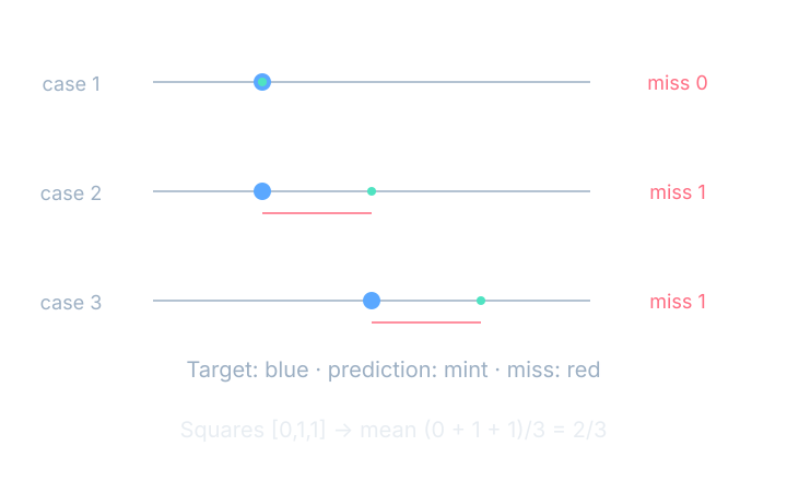
For numerical targets, mean squared error averages the squared differences between predictions and targets. Squaring prevents positive and negative misses from canceling. It also makes larger misses more costly: doubling a miss multiplies its square by four. The resulting units are the square of the target’s units, which matters when comparing datasets with different scales.

These scalar examples are separate from our classifier. They let us see the ruler without introducing another model. A prediction can be close without being exact, and an average can conceal which individual cases were poor. It is useful to inspect both the aggregate loss and some examples that contributed to it.

Let N be the number of examples, y the target, and y-hat the prediction. The superscript in parentheses selects an example rather than raising a number to a power. The square outside the difference is the actual squaring operation. The summation visits all N examples before the final division.

In words: square each prediction’s miss, add the squares, and divide by the number of examples.

An unlikely outcome carries more surprise

Classification asks a different question: how much probability did the model assign to the answer that occurred? An unlikely observed outcome should carry more surprise than a likely one. We want independent probabilities multiplied together to become surprises added together. A logarithm provides exactly that relationship.

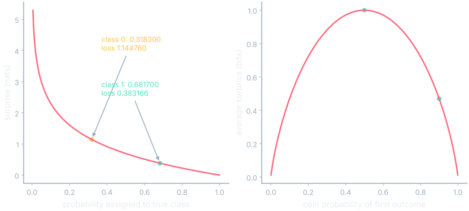
A logarithm asks which exponent produces a number in a chosen base. Log base two of eight is three because two cubed is eight. For probability one-half, negative log base two is one, because log base two of one-half is minus one. A bit is a base-two information unit. One bit of surprise corresponds to an outcome assigned probability one-half.

A nat is the information unit based on the natural logarithm, written ln. It is the inverse of the exponential with base e. Changing the log base changes the numerical scale of surprise, so a loss in nats cannot be compared numerically with the same quantity in bits without conversion. Our classifier’s cross-entropy uses natural logarithms.

Let p be the list of outcome probabilities and c select an outcome. Its surprise is weighted by how often that outcome occurs under p. The expression H(p) names the resulting entropy. This is uncertainty in the distribution, not a fraction of predictions that a classifier got wrong.

In words: weight each outcome’s surprise by its probability, then add.

An outcome with probability one carries zero surprise because it was certain under that distribution. As an observed outcome’s assigned probability approaches zero, its negative logarithm grows without bound. At exactly zero, the limiting penalty is infinite. A plot must not hide that limit by placing a finite point at the left endpoint.

Grade the model’s assigned probability

Return to the unchanged fixed model, input x=(1,0), and target class 1. A one-hot target selects one class with a 1 and puts 0 in every other entry. With class 0 first and class 1 second, the target is (0,1). Cross-entropy averages negative log probabilities using the target entries as weights.

Likelihood here means the probability the model assigns to the observed answer. Increasing that probability lowers its negative logarithm. We do not need to describe the bars as geometrically overlapping: the target selects a logarithmic penalty. Keeping that calculation explicit will make the derivative easier to follow than an analogy about overlapping shapes.

Let y_c denote the target entry for class c, and p_c the model’s assigned probability. The negative sign turns the nonpositive logarithm of a probability into a nonnegative penalty. A one-hot target leaves exactly one contributing term. A more general target distribution can weight several terms.

In words: multiply each log probability by the target’s entry, add, then negate; a one-hot label selects the correct class.

For the separate logits (2,1) example, class 0 costs −ln(e/(e+1))=0.313262 nats. Class 1 costs −ln(1/(e+1))=1.313262 nats. These numbers belong to that additional illustration, not our fixed model. Naming the input logits and target avoids accidentally borrowing a convenient loss from a different prediction.

See it move

Move the probability assigned to the true class toward zero, then toward one. Compare the logarithmic penalty with mean squared error against the one-hot target. Flip the label without moving the probabilities and watch which share now gets graded. The coin mode instead weights surprise by the coin distribution itself, producing entropy in bits.

The scalar mode returns to the three numerical predictions and targets. Editing a cell changes the corresponding miss before the average is recomputed. These modes show why “the loss” is incomplete information: we need the prediction type, target convention, averaging rule, and units to interpret its magnitude.

A surface over the weights

So far we have varied predictions directly. A training algorithm instead changes parameters that produce those predictions. Imagine trying many pairs of weights and calculating the loss at each pair. Each pair gives one height, forming a surface over weight space. The horizontal coordinates now name parameters, not input features.

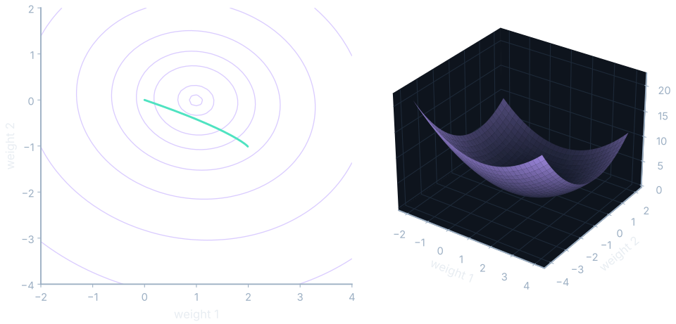
E1 has exactly two parameters, so its stored surface is the complete objective over those two directions. The contours and three-dimensional view use the same recorded array. Its actual parameter path is overlaid, and its final recorded loss is 0.006484. The source is E1.json’s stored surface and snapshots, with the final value in E1.summary.json.

This surface belongs to E1’s numerical fitting task. It is not the cross-entropy surface of our seventeen-parameter classifier. A larger model could only be shown through selected directions or slices in a three-dimensional picture. Rotating such a picture changes the view, not the number of parameter directions the picture contains.

Read the contour spacing as a clue to how rapidly the loss changes across the displayed plane. Equal-height curves close together indicate a larger change over a short horizontal distance than widely spaced curves. That picture prepares the next question: can we measure the local change with respect to each weight and choose a small move that lowers the loss?

Where this shows up when you train

For what these loss numbers look like across a real training run, see Reading the Graphs.

During training, a prediction may contain many entries while the loss supplies one scalar to differentiate. The objective must match what the task rewards. Numerical distance, probability assigned to a label, and a downstream task score need not be the same quantity. Record the loss formula and reduction convention alongside the run.

We have now graded the fixed model without changing it. The target remains class 1 and the original loss remains 0.383165978794 nats. Next we will measure how one weight affects that number, use the slope to choose an update, and recompute the prediction to check whether the step helped.

Where we’re headed

We have a score. Next we will measure which direction each weight must move to reduce it. Continue to the next chapter.