Use the stored forward values
The last layer’s gradients were short to calculate because its weights touch the logits directly. How does the loss reach a weight farther back? We will reuse the stored forward values and trace every returning contribution. The arithmetic will give one derivative beside every parameter, including the entries whose derivatives are zero.
Restore the original model from chapter 7. We are not starting from the output layer already updated in chapter 9. The input is still x=(1,0), the target is class 1, and the hidden values are (t,t,0). Resetting the starting state makes this a complete-model update that can be compared with the earlier last-layer-only update.
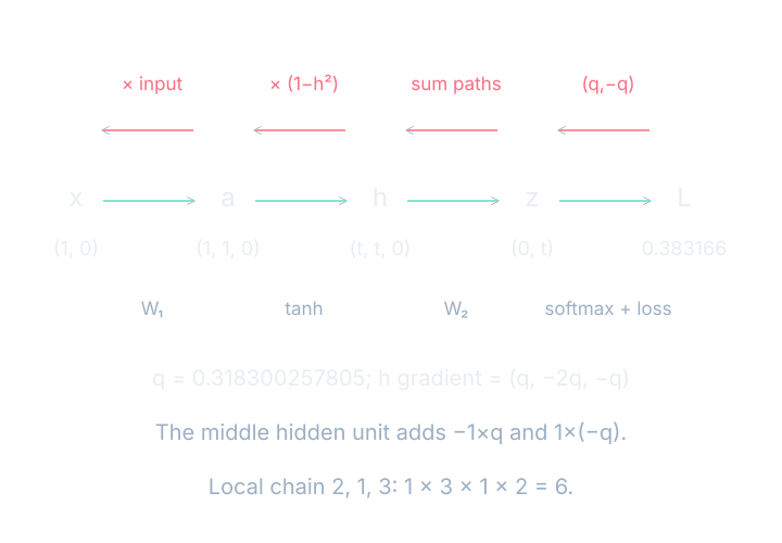
A computational graph connects individual operations by their data dependencies. The chain rule multiplies local derivatives along a path and adds contributions where paths meet. Backpropagation applies this rule backward through the graph. It uses forward values that have already been computed, so each operation has the information needed to calculate its local slope.
Think of the returning number as a sensitivity: how much the final loss would change for a small change in that intermediate value. A multiplication, addition, or activation converts that sensitivity into contributions for its own inputs. We are not sending a desired replacement activation backward. We are calculating how the existing computation responds to changes.
A chain before a branch
Take a teaching chain whose local multipliers are 2, 1, and 3. Starting from incoming derivative 1 at the end, the return calculation is 1×3×1×2=6. Each link scales the sensitivity it receives. Reversing the order of traversal does not reverse the meaning of the original forward calculation.
A branch adds another step to this picture. If one intermediate value influences the loss by two outgoing paths, changing it perturbs both paths. Its total derivative must include both effects. Dropping one outgoing connection would compute the gradient of a different graph, even if the remaining arithmetic looked internally consistent.
Put one gradient beside every parameter
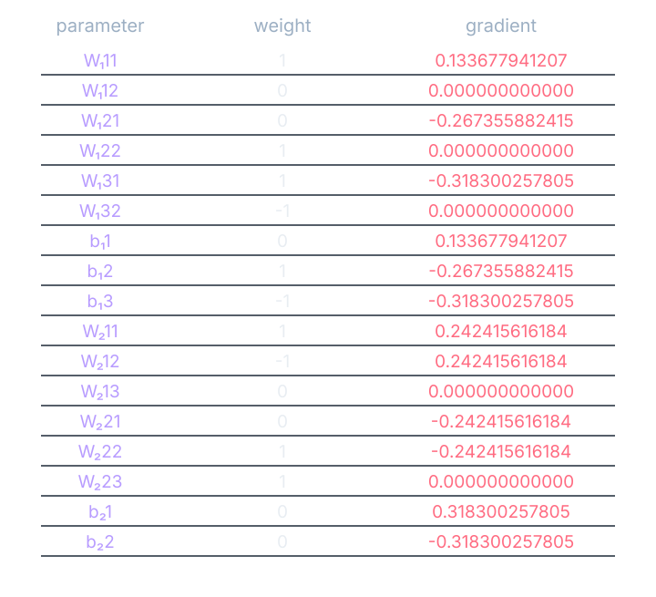
We can now align derivatives with the original parameter arrays. The W₁ gradient has three rows and two columns, just like W₁. The b₁ gradient has three entries, just like b₁. The same shape correspondence holds for W₂ and b₂. The backward pass does not invent a new parameter layout.
The complete gradient inventory
W₁ gradients are [[0.133677941207,0],[−0.267355882415,0],[−0.318300257805,0]]. The b₁ gradients are [0.133677941207,−0.267355882415,−0.318300257805]. W₂ gradients are [[0.242415616184,0.242415616184,0],[−0.242415616184,−0.242415616184,0]]. The b₂ gradients are [0.318300257805,−0.318300257805]. All seventeen entries are present.
An upstream gradient is the sensitivity arriving from later operations. A local gradient is one operation’s derivative with respect to an input. Multiplying them produces the contribution passed toward that input. The directional names follow the computation graph; they do not mean that data are physically moving backward through time.
Autograd is software that records operations and applies this same chain rule. It relieves us of manually expanding every derivative, but it still differentiates the graph we actually wrote. A mistaken input, missing dependency, or wrong loss definition can produce a perfectly consistent derivative of the wrong calculation.
See it move
Complete the forward pass, then select Trace backward. Choose the middle hidden unit’s input weight and inspect its two outgoing paths. Their products add before the tanh slope and input multiplier are applied. Select a zero-gradient entry and check which factor caused the zero. Both actions should agree with the full table above.
The tracer also perturbs the selected parameter on either side of its current value and recomputes the loss. That centered finite difference supplies an independent numerical check. Its last few digits can differ because the nudge and floating-point arithmetic are finite, but the sign and scale should agree away from problematic numerical limits.
Move the parameters together
We have calculated every derivative at the original parameter state. Now choose learning rate η, eta, equal to 0.1 and update all parameters from that state together. Do not update a hidden weight, recompute a downstream derivative with the changed model, and call the result one simultaneous gradient step. That would mix different starting states.
Apply every parameter update
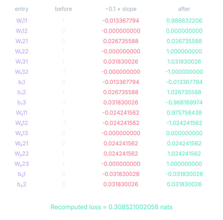
W₁ becomes [[0.986632205879,0],[0.026735588241,1],[1.031830025781,−1]], and b₁ becomes [−0.013367794121,1.026735588241,−0.968169974219]. W₂ becomes [[0.975758438382,−1.024241561618,0],[0.024241561618,1.024241561618,1]], and b₂ becomes [−0.031830025781,0.031830025781]. Each new value is its original value minus 0.1 times its own derivative.
The new preactivation is (0.973264411759,1.053471176483,0.063660051561). Applying tanh gives hidden values (0.750135303643,0.783152219713,0.063574194449). The third hidden value is now nonzero because its input weight and bias moved. That change can affect the output through its existing outgoing connections.
Recompute the complete pass
The new logits are (−0.102016225827,0.915725723919). The class-1 probability is 0.734532525343 and its loss is 0.308521002058 nats. Compare this with the original 0.383165978794 and the last-layer-only result 0.341413196910. These are different updates from the same original example, so their outcomes can be compared directly.
Backpropagation and the optimizer perform different jobs in this sequence. Backpropagation computes the derivative table. The optimizer uses that table, the learning rate, and possibly retained state to choose new parameter values. We can change the optimizer without changing the chain rule that computed the gradient.
Where this shows up when you train
For a new layer or loss, a small numerical example is a valuable debugging tool. Keep inputs, targets, and initial parameters fixed. Compare the forward values first, then the gradient arrays, then the simultaneous update. This separates a wrong forward recipe from a wrong derivative or a wrong update implementation.
The model now has a complete, inspectable learning step: forward values, loss, returning sensitivities, and updated parameters. Repeating that step over batches introduces progress counters, data ordering, and optimizer memory. Those are the next pieces we need before a long training trace becomes readable.
What you now know
- The chain rule multiplies local slopes along each path.
- Contributions add when several paths reach a value.
- Backpropagation computes the derivatives, and the optimizer changes parameters.
Where we’re headed
We have one complete update. Next we will organize many updates into batches and epochs. Continue to the next chapter.