Downhill: the Gradient · Training a Model, All the Way Down

Which direction lowers the loss?

We have a loss, a fixed model, and a target. Which weight should move, and in which direction? We will measure the local effect of a small change, collect those effects into an arrow, and take one checkable update. Then we will recompute the loss instead of assuming the update succeeded.

A derivative is the local rate of change of an output with one input. A partial derivative varies one parameter while holding the others fixed. A gradient collects those partial derivatives into a list with one entry per parameter. In a two-weight picture we can draw that list as an arrow in weight space.

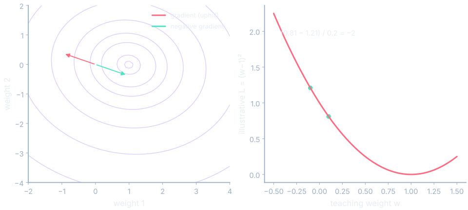
The gradient points uphill locally; the update moves in the opposite direction.

The gradient points uphill locally: it indicates the direction of steepest increase under the usual Euclidean distance convention. Its negative points downhill. Neither arrow has knowledge of every distant point on the surface. The direction describes the neighborhood of the current weights, so it changes as the weights move.

A local minimum is no higher than nearby points. A saddle has rising and falling directions. A plateau has small slopes over a region. These shapes help us describe why a local update might slow down or behave differently across directions. They do not turn a single two-dimensional picture into a complete map of a larger model.

Estimate a slope by two nudges

For the teaching slice L(w)=(w−1)², evaluate near w=0. L(0.1)=0.81 and L(−0.1)=1.21. The centered finite difference is [0.81−1.21]/0.2=−2. The negative sign says increasing w slightly lowers the loss here. This illustrative slice is a different objective from E1’s recorded surface.

A finite difference estimates a slope from evaluated changes rather than symbolic differentiation. The centered version looks on both sides of the point. It is useful for checking an analytic calculation, though rounding makes extremely tiny nudges unreliable. Later, we will use it as an independent check on every parameter in our small model.

Follow loss back to one output weight

Return to the fixed model’s original parameters, input x=(1,0), and target class 1. We have hidden values (t,t,0), where t=0.761594155956. Let q=p₀=0.318300257805. Since the two probabilities sum to one, the difference between class 1’s probability and its target value is p₁−1=−q.

From loss to one output weight

For softmax followed by cross-entropy, the loss derivatives with respect to logits are dL/dz=(p₀,p₁−1)=(q,−q). The first logit depends on W₂₁₁ through hidden value h₁=t. Thus dz₀/dW₂₁₁=t, and dL/dW₂₁₁=q×t=0.242415616184. The corresponding weight in the second output row has gradient −q×t.

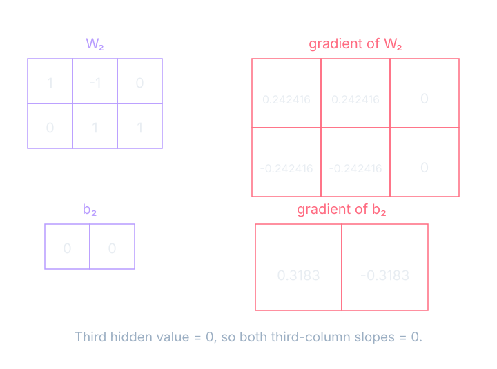
The 2 by 3 output-weight gradient has rows (0.242416, 0.242416, 0) and (−0.242416, −0.242416, 0). The bias gradients are (0.3183, −0.3183); the zero hidden input produces the zero third column. — Each output weight receives the score error multiplied by its hidden input.

The full W₂ gradient is [[0.242415616184,0.242415616184,0],[−0.242415616184,−0.242415616184,0]]. The b₂ gradient is [0.318300257805,−0.318300257805]. The two third-column entries are zero because the hidden input h₃ is zero. We have not omitted those entries; zero is their computed derivative for this example.

Let c select a class and j select a hidden input. The output score’s error signal is p_c−y_c, and its multiplier with respect to that weight is h_j. Multiplying them gives one entry of the weight gradient. The bias derivative has the same score signal because the bias enters its score with multiplier one.

$$ \frac{\partial L}{\partial W_{2,cj}}=(p_c-y_c)h_j $$

In words: the output score’s error signal times the hidden input gives that weight’s slope.

Changing one logit changes every probability through softmax’s shared denominator. The compact p−y result already accounts for that coupling when cross-entropy is differentiated. Treating the probabilities as independently adjustable outputs of separate score functions would miss part of the calculation. The derivative follows the actual recipe used to produce the loss.

Take a step and check the result

The learning rate η, pronounced eta, sets the scale of the update. Gradient descent subtracts the learning rate times the gradient. For this demonstration choose η=0.1 and change only the output layer. The hidden weights and biases stay at the original initialization so that we can isolate the effect of the last-layer gradients.

Update the output layer together

W₂ becomes [[0.975758438382,−1.024241561618,0],[0.024241561618,1.024241561618,1]]. The new b₂ is [−0.031830025781,0.031830025781]. Every new entry uses its own original value and its own gradient. For example, 1−0.1×0.242415616184=0.975758438382 after rounding.

Let w stand for one parameter and the partial derivative name its slope. The left arrow means replace the stored value with the expression on the right. For a full update, we apply the same rule to every selected parameter using gradients computed at the same original model state.

$$ w\leftarrow w-\eta\frac{\partial L}{\partial w} $$

In words: subtract the learning rate times the slope from the current weight.

Check the prediction after the step

The hidden values remain unchanged. The new logits are (−0.068754489100,0.830348645056). Softmax gives p₁=0.710765161555, and the class-1 loss becomes 0.341413196910 nats. The old loss was 0.383165978794 nats. The probability assigned to the true class increased and the loss decreased.

A successful small step does not prove that any larger step would help more. The derivative describes local behavior. Moving far enough can cross the valley and climb the other side, or enter a region with a different slope. We therefore look at recorded paths produced by different update settings on the same objective.

Three recorded optimizer paths overlay loss contours with weight 1 horizontally and weight 2 vertically. Each panel labels its optimizer, learning rate, and recorded status. — Different step rules and rates produce different recorded paths on the same objective.

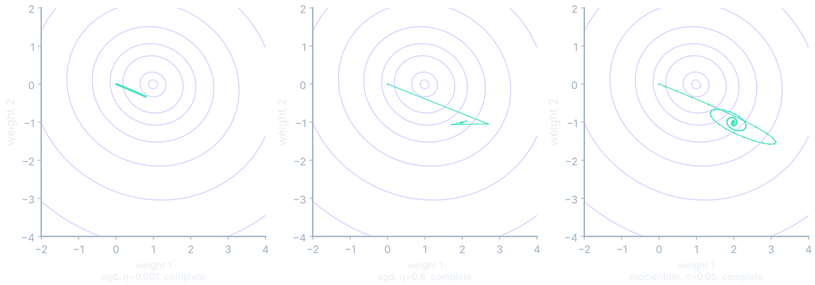
These paths come from E1’s stored comparison traces. Their starting weights and objective agree, while their recorded optimizer choices and learning rates differ. Keep their actual statuses and any path that leaves the visible area. A diagram clipped to a convenient range must not silently replace a large recorded value with an invented in-range point.

See it move

Scrub the primary E1 path first. Then choose an available recorded comparison. The separate sandbox computes its own trajectory from E1’s stored input and target values. Because those values are rounded in the exported file, sandbox arithmetic is labeled separately from the original recorded run. Its learning-rate and momentum controls never relabel a recomputed path as a measurement.

The nudge readout shows the centered finite-difference calculation at the selected point alongside the analytic gradient. Inspect both coordinate directions. The contour and rotated surface use the same stored loss grid; rotating the picture changes your view while preserving the underlying values. Keep the uphill gradient distinct from the downhill update direction.

Run a line fit yourself

We can now train a model small enough to print every parameter and derivative. E0 fits y=ax+b to twelve points using two parameters, a and b. The source data and runner are shipped with the repository. This is a function-fitting exercise on the same points used to evaluate its loss, so it demonstrates optimization rather than held-out performance.

A gradient measures local change and a checked update can reduce loss.

nice -n 19 .venv/bin/python -m trainkit fit trainkit/samples/fit.csv --output fit-output

The recorded final values are a=1.985458, b=0.999998, and loss=8.3e-05 after sixty steps. The summary sources point to E0’s recorded parameters and loss series. Read the printed changes as applications of the update rule: a slope, a chosen rate, and a new value whose prediction can be checked.

The same samples can be run through the experiment wrapper with python experiments/run_E0.py from the archive’s parent. The two routes serve different packaging needs, but the teaching objective remains the same: make each parameter update visible. A smaller in-sample loss establishes that the fit improved on those points, not that it will behave well everywhere.

Where this shows up when you train

A finite-difference nudge is a useful diagnostic when implementing a new calculation. Check several nudge sizes and compare both signs and magnitudes with the analytic derivative. Too small a nudge can disappear into rounding; too large a nudge measures behavior over a wider interval rather than a very local slope.

We have only updated the last layer so far. The hidden layer also contains parameters, and their effect reaches the loss through several operations. Next we will carry the same error signals backward through those operations, adding all returning paths until every one of the seventeen parameters has its own derivative.

What you now know

A gradient is a list of local slopes.
Gradient descent subtracts a scaled gradient.
Recomputing the loss checks what the update actually did.

Where we’re headed

The output layer is now accounted for. We will follow the same error signal through the hidden activation to every earlier parameter. Continue to the next chapter.