The Training Loop

One update has several stages

One update changed the fixed model’s prediction. What turns that calculation into a training run? We repeat the stages over examples, keep track of progress, and record enough state to understand each step. The arithmetic inside a stage remains familiar even when the surrounding loop becomes longer.

A mini-batch is a subset of examples used for one update. A step is one optimizer update. An epoch is one training-set’s worth of consumed examples. Those counters describe different things: a large dataset divided into small batches can require many steps to complete one epoch. The last batch can be shorter without disappearing from the accounting.

Shuffle means changing the order of training examples, often between passes. Stochastic gradient descent estimates the gradient using sampled examples rather than evaluating the full training set for every update. Full-batch descent uses all training examples. The choice changes the amount of work per step and the variation in the gradient estimates.

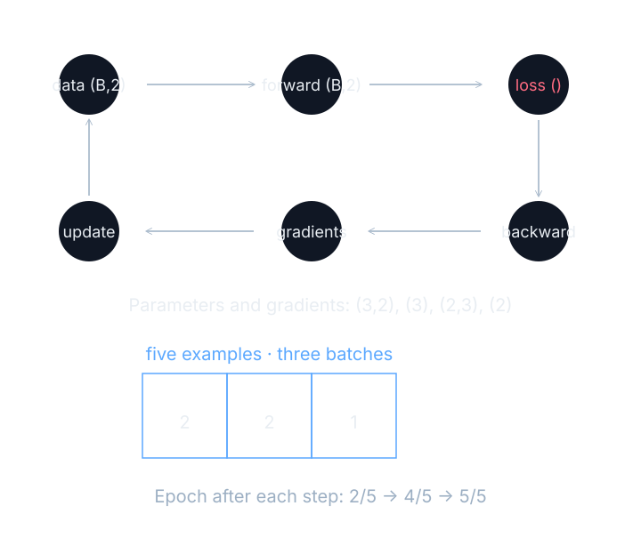
The diagram keeps the fixed model’s parameter shapes attached to the loop: (3,2), (3), (2,3), and (2). A batch enters the forward pass, the loss reduces predictions to a scalar, the backward pass computes matching gradient arrays, and an update changes the parameters. The next batch then uses those new values.

A batch loss and a whole-split evaluation loss need not be the same number. The batch might contain easier or harder examples than the full set, and its loss might be measured before rather than after the update. A useful run record states which examples and parameter state each reported quantity uses. A chart labeled only “loss” leaves those choices ambiguous.

The gradient does not determine the step alone

An optimizer turns gradients and retained state into updates. Plain gradient descent needs the current gradient and learning rate. Momentum retains part of earlier directions. Adam, adaptive moment estimation, retains averages of gradients and their squares. These rules can receive the same gradient and still produce different parameter changes.

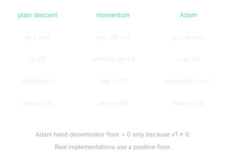
Use a single illustrative weight w=1 and gradient g=1. With learning rate η, eta, equal to 1/2, plain descent gives w_new=1−(1/2)×1=1/2. This is an optimizer-state illustration, not a second neural network. Keeping the arithmetic separate prevents us from confusing its one-digit values with the fixed model’s recorded gradients.

For momentum, let the old velocity v=1 and retention m=1/2. We use the unnormalized convention: new velocity equals retained old velocity plus the current gradient. Thus v_new=(1/2)×1+1=1.5, and w_new=1−(1/2)×1.5=1/4. The retained state made this step larger than plain descent’s step.

In words: retain part of the previous velocity, add the current gradient, then step using the new velocity.

The subscript k counts updates. The previous velocity is v with subscript k−1; g_k is the new gradient. Other conventions scale the incoming gradient too, so the word momentum by itself does not determine the arithmetic. A reproducible description includes the exact update rule and its retention setting.

Let r retain part of the gradient mean and q retain part of the mean square. The square on g_k changes what information the second average stores. It records magnitude without sign, while the first average can combine positive and negative gradients. We give these states different names because they play different roles in the final division.

In words: average the gradient and its square separately.

The hat marks the averages after correcting for their initial zeros. The denominator contains the square root of the corrected mean square plus a small positive floor δ, pronounced delta, in real software. Our hand example used zero only because the denominator was already nonzero. It is not a recommendation to remove the numerical floor from an implementation.

In words: correct the initial zero averages, then scale the average gradient by the square root of its average square plus a small numerical floor.

Adam’s actual update magnitude is not generally the learning rate times the raw gradient norm. Retained averages and coordinatewise scaling intervene. This will matter when we read an update-to-weight ratio: the safest source is the actual parameter change, not an expression that assumes plain gradient descent.

Rate, decay, clipping and checkpoints

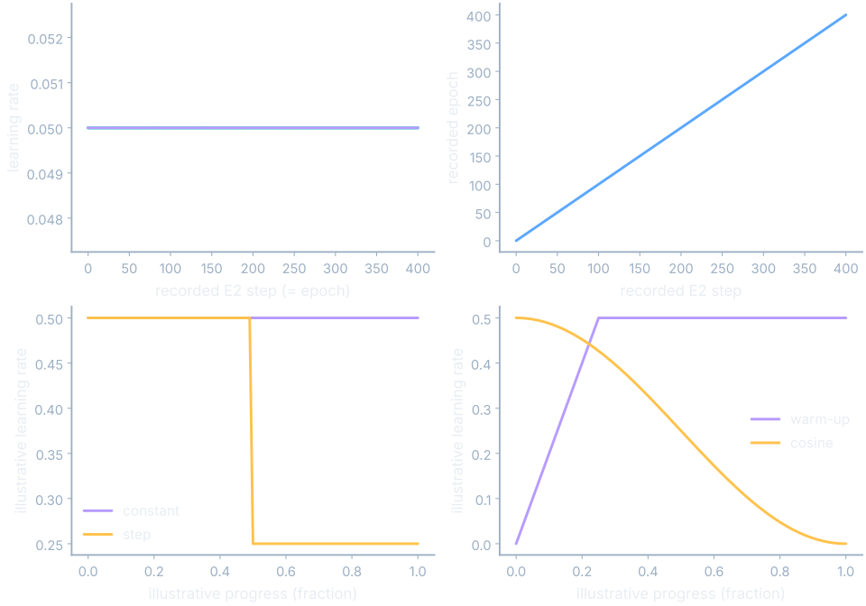
A learning-rate schedule changes η as training progresses. Warm-up increases the rate during an initial interval. A schedule can instead stay constant, drop at chosen points, or follow a smooth curve. Those are chosen rules; the presence of a smooth-looking loss curve does not tell us which schedule was used.

Weight decay shrinks parameters toward zero under a specified rule. Gradient clipping limits gradient magnitude before the optimizer uses it. A checkpoint saves model values at a named step. Continuing the same optimizer trajectory also needs its retained state and other run state; the book’s JSON parameter snapshots do not contain a complete optimizer-resume checkpoint.

The main recorded learning-rate trace in the figure is E2’s constant schedule. The step, warm-up, and cosine insets are labeled illustrations. Snapshot markers indicate actual saved states, not every visually interesting point on the loss curve. We keep those two kinds of evidence separate so a reader can tell which state can actually be reopened.

Clipping is not evidence that the unmodified gradient was incorrect. It is a deliberate restriction on the update input. Likewise, decay changes the optimization recipe rather than redefining the forward pass. A run’s settings should record whether these operations were enabled and where they occurred relative to the stored diagnostic values.

Replay a recorded loop

E2 is a recorded full-batch run. Its batch is its complete training set, so every update consumes one epoch’s worth of examples. It does not use the five-example teaching strip or a proposed four-example animation. The replay must read E2’s actual epoch values rather than deriving a more cinematic story from unrelated batch sizes.

See it move

Begin paused at initialization. Step once and inspect a parameter’s old and new values. The gradients shown for an update are pre-update batch gradients, while the displayed loss and parameter state are post-update. Keeping that timing distinction visible lets us ask which gradient produced a change instead of comparing quantities from incompatible moments.

Select a sample in the logits view and inspect its input and probability shares. Then move the transport cursor. The scalar loss, parameter snapshot, and available sample values follow recorded progress. Sparse panels report the step they actually contain; they do not invent intermediate arrays just because the scalar trace has a finer cadence.

The run loader also accepts a local trainkit run.json. The file stays in the browser and is checked before it is used. Missing fields show as not recorded, while measured zeros remain zeros. That distinction matters especially at initialization, when a zero diagnostic can be a placeholder for work that has not been computed yet.

Where this shows up when you train

The loop’s stages recur across model families. Their input structures and forward calculations differ, but we still need an objective, derivatives, an update rule, and progress records. Recognizing that common structure makes a convolutional network or sequence model less like a separate training ritual and more like a new forward recipe inside a familiar loop.

A run is more than a final weight file. Its trace explains how the parameters changed, which examples were evaluated, and which states were saved. Next we will read the shapes of those traces, comparing falling loss with the task score and the checkpoint that was actually kept.

Where we’re headed

The next chapter shows what these measurements look like across recorded training runs. Continue to the next chapter.