What shape does it eat?
Move a handwritten digit one pixel to the right. The bright pixels now occupy different input slots, but we would usually like to recognize the same digit. How can a model reuse something it learned at one location elsewhere in the image? We’ll put the local window calculation from loops to matrices inside the training loop.
A convolutional neural network applies shared local filters over a grid. A channel is one aligned grid of input or feature values. A filter is a small array of weights that combines a local patch across those channels. Our input digits have one brightness channel, so a batch enters as (batch,1,8,8). The rows and columns really are neighboring locations; their order is part of the model’s assumption.
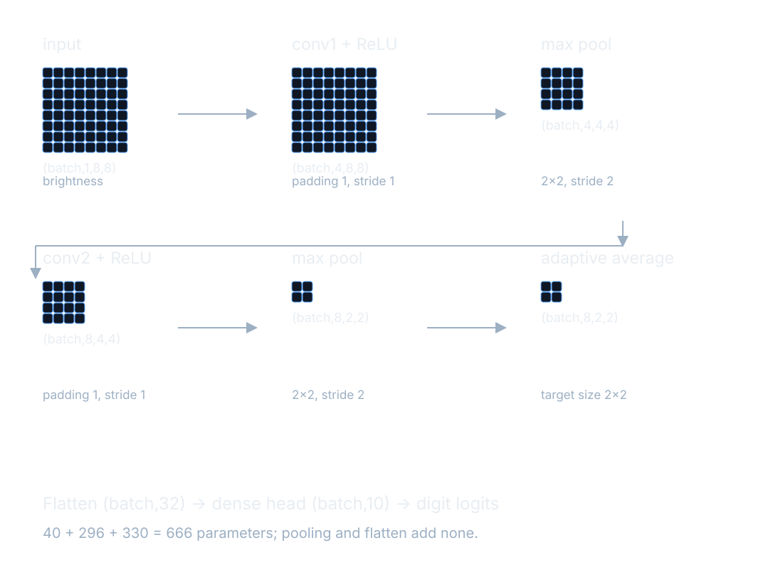
E4’s first convolution makes four channels on the 8×8 grid. ReLU follows, then max pooling reduces the spatial grid to 4×4. The second convolution mixes those four input channels into eight output channels. Another ReLU and pool produce (batch,8,2,2). Adaptive average pooling to (2,2) retains that size here. We then flatten the array into 32 ordered values per example and apply a dense layer to make ten digit scores.
One rule visits every location
weight sharing means we reuse the same parameter at multiple positions. A filter does not acquire a different rightmost weight when its window moves to the next column. That forces the network to use one local rule across the grid. A receptive field is the set of input locations that can influence a particular output. Later layers can gather information from a wider area because their inputs already summarize smaller neighborhoods.
pooling summarizes neighboring responses into fewer entries. Max pooling keeps the largest value in a patch. It can preserve a strong response even when that response moves within the patch, but crossing a pooling boundary can change the answer. A stride is the distance between consecutive window positions; padding supplies values outside the original image so that edge locations can participate in a chosen way.
Compute the filter cells
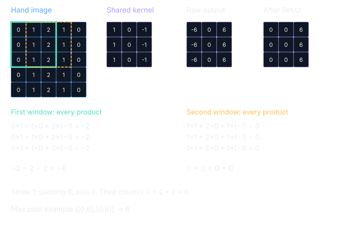
Our hand image has five identical rows: [0,1,2,1,0]. The kernel has three identical rows: [1,0,−1]. We use stride one, no padding, and zero bias. The output has three rows and three columns because the 3×3 window fits in three positions along each input axis. These values are chosen for arithmetic; they are not saved learned kernels.
Two full filter cells
At the first output, the top patch row contributes 0×1+1×0+2×(−1)=−2. The next two rows have the same three products, so the output is −2−2−2=−6. Move one column right. Each row now contributes 1×1+2×0+1×(−1)=0, and the output is 0+0+0=0. Move right again: each row gives 2×1+1×0+0×(−1)=2, so the result is 6.
Every vertical placement meets the same row pattern. The complete output therefore has three identical rows [−6,0,6]. ReLU changes each to [0,0,6]. Call the image entries X, the kernel entries K, and the feature-map entries F. The indices i,j locate an output; a,b range over the kernel offsets:
$$F_{ij}=\sum_{a,b}K_{ab}X_{i+a,j+b}$$In words: multiply the patch by the shared filter entry by entry, then add the products; add the filter’s bias afterward if present.
A pooling cell
The 2×2 response patch [[0,6],[0,6]] becomes max(0,6,0,6)=6. Pooling chooses a value rather than multiplying by a new learned row. Keep the raw filter result, the activated response, and the pooled result separate when explaining a prediction. A negative raw response can become zero at ReLU before any pooling occurs. The widget exposes the full product list, preactivation, and final activation for a selected output location.
Replay filters as the model trains
Training now adjusts the filter entries and the dense head together. The labels grade the final digit probabilities; they do not directly tell an early filter to become a vertical edge detector. An early weight receives its gradient through all the intervening operations. This is the same backward computation we studied earlier, applied to a different arrangement of shared parameters.
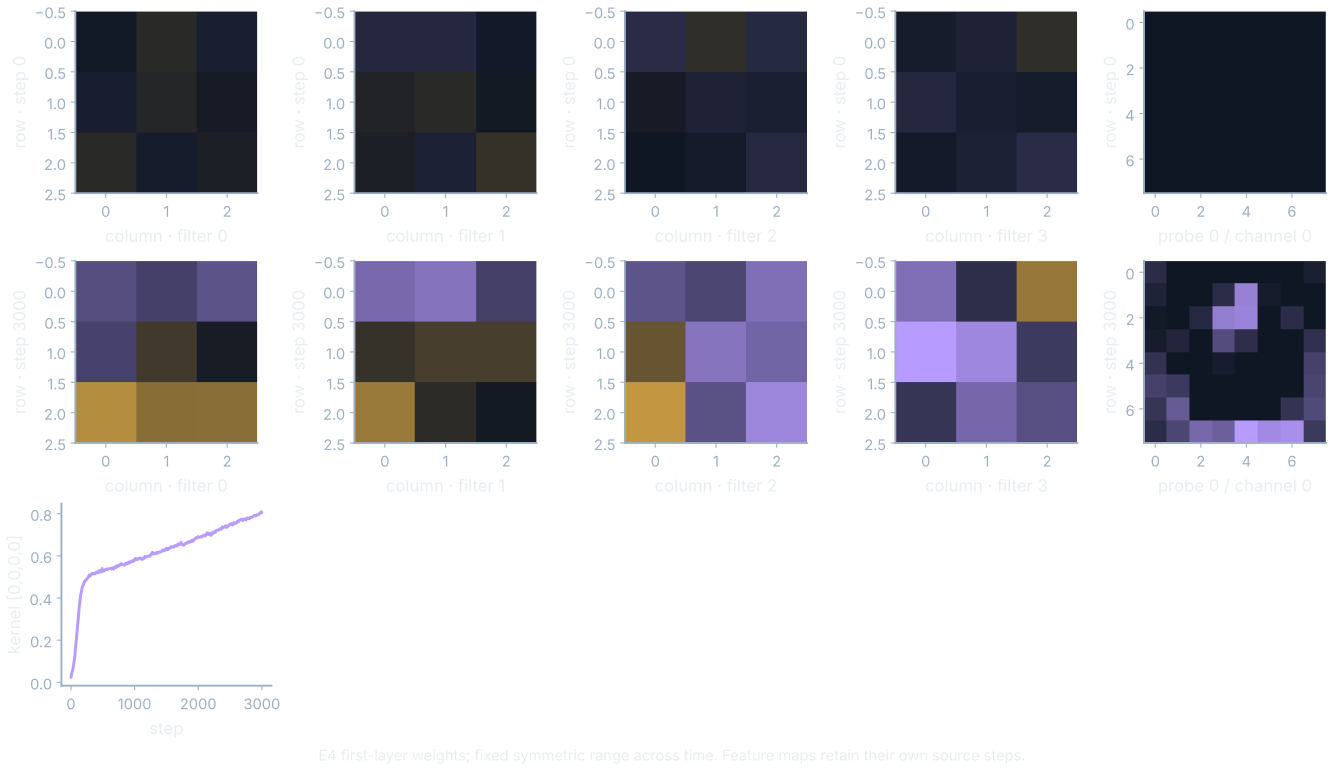
E4’s final optimizer step is 3000. The saved training loss is 0.008242, validation loss is 0.128412, and validation accuracy is 0.961474. They come from media/runs/E4.summary.json#/values/final_loss, /values/final_val_loss, and /values/final_val_accuracy, pointing to the corresponding run series at index 3000. A good classification rate can coexist with a noticeable loss gap because loss also measures how confidently probabilities are assigned.
Where this shows up when you train
The final confusion matrix counts observed mistakes. Read its rows as true digit labels and its columns as chosen digit labels. Diagonal entries count correct predictions. The final correct counts by class are [58,58,57,58,59,58,59,58,52,57], from media/runs/E4.summary.json#/values/confusion_diagonal, whose run pointer is /meta/headline/confusion_diagonal. The row totals matter too; a count alone is not a per-class success rate.
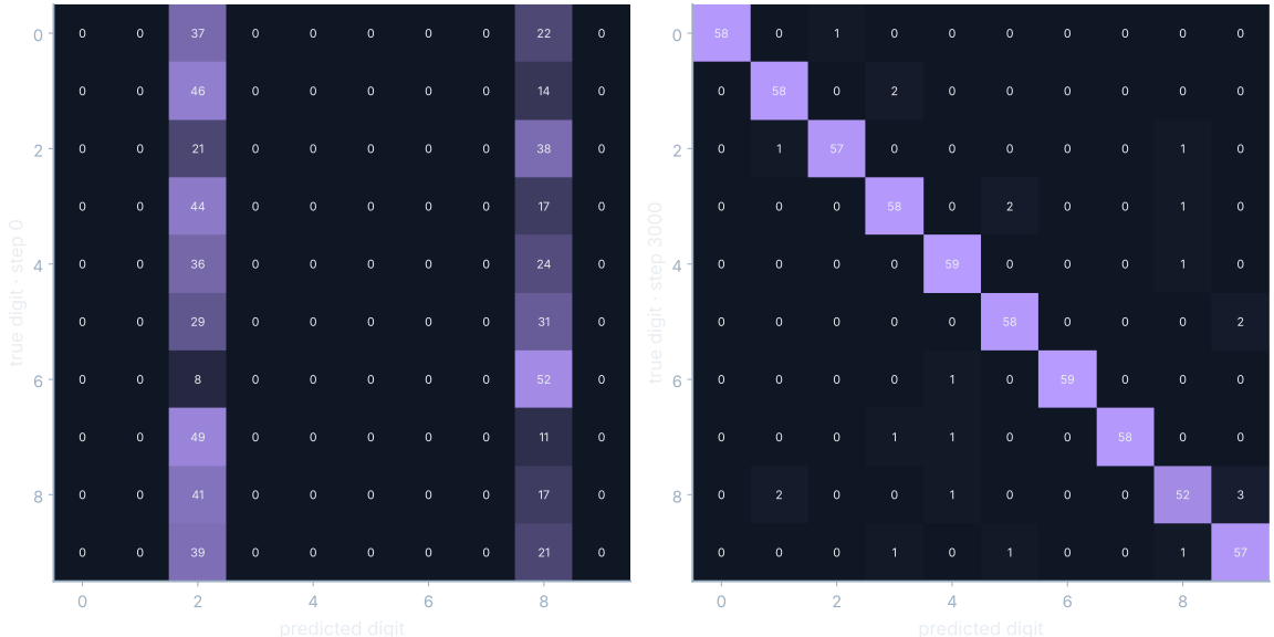
An off-diagonal cell is an actual error category from this validation split. It gives us a place to investigate without inventing a dramatic failure image. We can compare initial and final counts on the same scale and see which mistakes decreased. We should still inspect individual examples before attributing an error to a particular stroke, filter, or preprocessing choice.
Convolution fits images and other grids where local adjacency carries meaning. It can be inappropriate for an ordinary table whose adjacent columns are unrelated measurements. Swapping such columns should not create a new spatial relationship. Choose the architecture because its sharing rule matches the data’s structure, then verify the result on an appropriate split. Here the remaining observed errors and the recorded loss gap are part of the result we keep, alongside the successes.
What you now know
- A convolution shares a local filter across a grid.
- Feature maps and pooling preserve or reduce spatial structure.
- A confusion matrix records specific errors that accuracy alone hides.
Where we’re headed
A sequence needs a shared rule too, but its next state also depends on the state it is carrying. Continue the story.