Getting Data into Tensors

Start with the examples

Our model needs arrays, but our data arrives as a file full of rows, images, or measurements. Which entries belong together, which one is the answer, and which information will be available when we predict? These decisions happen before the first gradient. We’ll make each conversion small enough to inspect and preserve a route back to its source.

A sample is one example used as input or evaluation. A feature is a measured or encoded input value. A row can be a sample without every column being a feature: the target must be separated before constructing inputs. An identifier can also be useful for splitting without being a useful prediction feature. Ask what each column means before converting everything that looks numeric into a tensor.

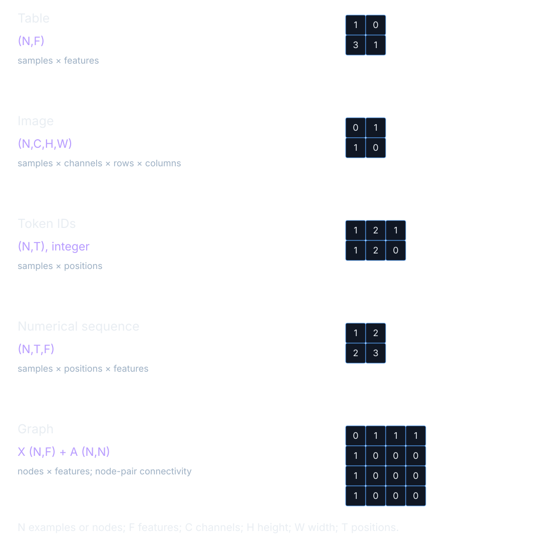
Read the axes aloud. A table X has shape (N,F): N samples, F features. Images have (N,C,H,W): samples, channels, height, width. Token IDs have (N,T), with T counting sequence positions. Numerical sequences have (N,T,F). Graphs combine node features X=(N,F) with adjacency A=(N,N). Here T is a sequence length, not softmax temperature. The same letter can carry a local meaning only when we state it.

Keep information in its proper split

The training split fits the weights. Validation guides development choices. A test set is reserved for the final assessment after those choices are complete. leakage occurs when evaluation information enters fitting or selection. This includes preprocessing statistics as well as model updates. If we compute a mean on the whole file and then split it, the training representation already contains information from the evaluation rows.

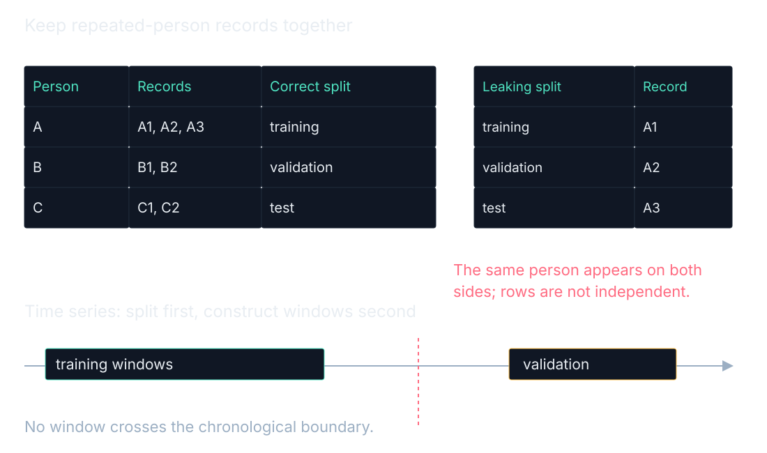
Independent rows are an assumption, not a consequence of storing data in a CSV. Repeated observations from the same person or device can be strongly related. Keep such groups together when evaluating transfer to new groups. For future prediction, split chronologically. stratification preserves class representation in a random split, which can be useful, but it does not replace grouping or time order. The right split follows the question we want the evaluation to answer.

Make the representation explicit

standardization subtracts the training mean and divides by its training standard deviation. normalization is the broader idea of transforming values to a chosen numerical scale or convention. These words can describe different operations, so our export records the actual recipe. We use m for the training mean, s for the training standard deviation, x for a raw value, and z for the transformed value:

The numeric ledger preserves a feature’s name, whether it was treated as numeric, its fitted mean, and its fitted scale. Category columns preserve their training vocabulary instead. The runner stores this preprocessing in model.json because the weights expect exactly that input representation later. Reordering categories or changing a numeric scale can change every weighted sum even when the exported weights are identical.

In words: subtract the training mean and divide by the training standard deviation; handle constant features explicitly.

The mask says which positions are real inputs for the relevant operation. It is separate metadata, not a guarantee that a zero-valued feature should be ignored. A legitimate pixel can have brightness zero and still matter to a convolution. Likewise, a graph needs its connectivity in addition to node features. If we keep only the feature matrix, the message-passing neighborhood has disappeared even though every node still has numbers.

Inspect each conversion

Start with the three-row CSV and use the first two rows for training. The length feature uses their mean and scale; the third row is transformed afterward. Select a numeric output to trace it back to its CSV row and column. Then change the training-row count and watch both numeric statistics and category vocabulary change. A split choice affects the representation, not just the rows used for the loss.

Where this shows up when you train

augmentation makes modified training examples intended to preserve the target’s meaning. A slight image shift can be appropriate when the class should survive that shift. It can be inappropriate when position itself defines the label. Define the allowed transformation using the task before making extra examples. Keep all versions of an original example in its training group, rather than allowing a transformed copy to leak into validation.

More rows do not necessarily provide more independent evidence. A thousand near-duplicate frames can describe less variation than a smaller collection from distinct conditions. A random split can hide that problem by placing nearly identical records on both sides. Inspect group identifiers and time ranges, not just split percentages. The arithmetic of the model cannot repair a misleading evaluation boundary chosen before training began.

Where we’re headed

We can now choose the objective, model, update settings and stopping rule for a concrete run. Continue the story.