Shaping a Problem for the GPU

What repeats, and what is shared?

A mathematical problem rarely arrives with its tensor layout already chosen. We have to decide what repeats, what is shared, and what depends on an earlier result. Shape design means making those choices explicit as axes and lengths. We will use the operations from the previous chapter to turn that question into a repeatable procedure.

Begin with the first layer of our fixed model. Its weight array has three rows and two columns. Give it two examples, (1,0) and (0,1). Each example meets the same three rows of weights. The example index names independent repetitions; the feature index names contributions to be added; the output index names the three units we produce for each example.

Write the input shape as (2,2): two examples, two features each. The weight shape is (3,2): three output units, two feature multipliers each. The output shape is (2,3): two examples, three results each. The repeated feature length must agree between input and weights because each dot product matches those entries one for one.

Let i select an example, j select a feature, and k select an output unit. The indexed rule is “sum over j of XᵢⱼWₖⱼ, then add bₖ.” Only j is reduced. Keeping the index meanings explicit is more useful than memorizing an unlabeled pattern of dimensions, especially when the same length happens to occur on several axes.

In row-major storage, the last axis varies fastest. Placing frequently traversed features next to one another can help the dot products read efficiently. However, contiguity alone does not identify the fastest implementation. The numerical library’s supported operations, tiling, temporary storage, and access pattern also matter. We choose a clear shape contract first, then measure a suitable implementation.

A polynomial is a table of repeated features

Fitting a polynomial gives us another way to find shared features. A polynomial combines powers of an input with coefficients. For a line, the two features are the constant 1 and the value x itself. The same coefficient pair is used for every example; changing the coefficients changes every prediction through that shared rule.

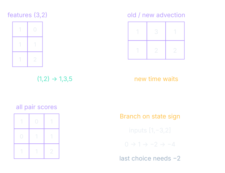
Use x=0,1,2 with targets y=1,3,5. The feature rows are [1,0], [1,1], and [1,2]. Coefficients (1,2) give 1,3,5 by dot products. Fitting means choosing coefficients to reduce a mismatch between predictions and targets. Least squares chooses coefficients to minimize the sum of squared prediction misses.

The normal equations group sums of products of features and targets into a smaller coefficient problem. They are useful here because we can inspect every number. They are not a universal recommendation for solving a numerical fit: their construction can amplify sensitivity to rounding when feature directions are nearly redundant.

Here b is the constant coefficient and a is the coefficient multiplying x. Their ordering follows the feature columns [1,x]. Reversing the coefficient list without reversing the feature columns changes the prediction. This is another instance of the shape lesson: a length-two vector is not fully described until we know what its two positions mean.

Some axes repeat; time may still wait

Advection means transport across space. A grid update often repeats the same local rule across many positions, making spatial locations candidates for parallel work. Time can still remain sequential: the next grid depends on the previous grid’s results. A tensor can therefore contain both independently repeated work and a dependency that additional lanes cannot remove.

This is an illustrative stencil, a rule that reads a fixed neighborhood. It is not a verified description of a production weather model. Its useful lesson is the dependency: we can calculate the cells of one new row together, but the following time step needs that row to be complete. Copying a familiar grid shape does not establish that two physical models use the same update.

This is only a comparison table. Later, attention will give learned comparisons a particular role in a model. For now, the array structure is enough: every row position meets every column position. If examples have different lengths, padding adds extra entries to reach a common size, and a mask specifies which entries must be excluded from meaningful work.

Chunking processes manageable groups while respecting such dependencies. We might batch many independent sequences, each with its own state, or divide a long sequence into pieces with state passed between them. That changes organization and memory demands. It does not license us to treat a state-dependent branch as an independent output cell.

How much work per byte moved?

Arithmetic intensity counts arithmetic operations per byte moved under a stated traffic model. Achieved performance divides arithmetic work by elapsed seconds. A roofline compares that achieved rate with two guides: a compute ceiling and a memory-transfer ceiling. At low intensity, movement can limit performance; at higher intensity, arithmetic can become the limiting resource.

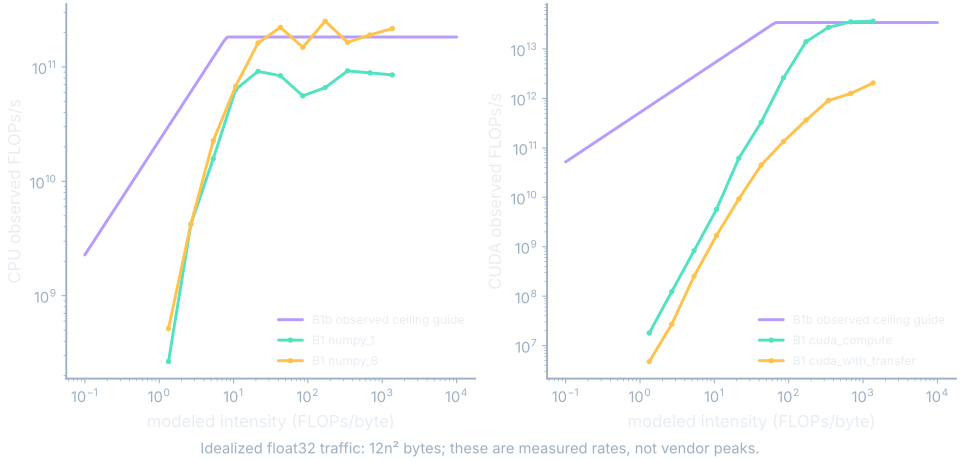
For square float32 matrix products of side n, use approximate work 2n³ and idealized minimum traffic 12n² bytes. There are two input matrices and one output matrix, each with n² four-byte entries. Dividing gives modeled intensity n/6 FLOPs per byte. This is an explicit traffic model, not a measurement of actual cache transfers or device traffic.

B1 supplies the plotted achieved points through its recorded sizes and elapsed times. B1b separately supplies observed ceiling rates. Keeping the sources distinct matters because the recorded settings differ. The CPU and CUDA panes each use their own ceiling guides; we do not apply the device’s bandwidth to a CPU point.

A tera-FLOP is a trillion arithmetic operations, and a gigabyte here is a billion bytes. Those prefixes make the rates readable; they do not change the underlying calculation. A roofline can help identify which resource to investigate, but the quality of its conclusion depends on its byte model and on whether the measured operation matches the problem we intend to run.

Where this shows up when you train

Use the designer to state sizes and assign axis roles. Begin with independent examples, shared features, and output units. Try a sequential time role and name the state that one time step passes to the next. The most valuable output is often the explanation of a dependency, even before we calculate a large operation count.

See it move

A matching B1 timing exists only for a recorded square matrix or matrix-vector product. The layer, stencil, and branch recipes include work that those intervals did not measure. The designer therefore reports unmatched recipes explicitly. If you supply your own measured work, bytes, seconds, and ceiling rates, its roofline view labels them as reader-supplied quantities.

When designing a training calculation, identify the repeated example, the shared parameters, and the per-output reduction. Estimate intermediate storage as well as arithmetic. Then preserve the dependency graph while choosing a layout and operation the numerical library can execute efficiently. We now have enough structure to follow one complete model prediction without leaving any of its numbers hidden.

Where we’re headed

We have shaped the work. Now we will follow the fixed model’s actual numbers from input to prediction. Continue to the next chapter.