What shape does it eat?
Two spirals wind around the same center. Can we tell which arm a point belongs to using only its two coordinates? We already know how to multiply a matrix, apply a bend, and update weights. Let’s use those operations to build a boundary that follows the data.
A dense layer connects every output to every input in the preceding layer. A multilayer perceptron stacks those layers with activations between them. “Dense” describes the connections. The points themselves can be spread far apart. A decision boundary is the set of input locations where the selected class changes. In our two-class problem, the boundary separates regions assigned to class zero and class one.
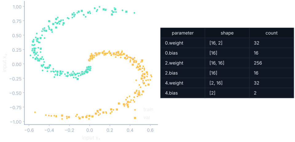
Each point gives us one row with two features. The row’s label is kept separately so that the model cannot read its answer as an input. E3’s recorded model has widths 2→16→16→2. Its weight arrays have shapes (16,2), (16,16), and (2,16), with a bias for every output at each stage. The hidden arrays give a point more coordinates to work with before reducing it to two scores.
Move the space before drawing the line
A straight boundary in the original plane cannot follow both interleaved arms. Instead of asking the final decision to become complicated, we can change the space it sees. Each hidden layer remixes the coordinates, shifts them, and bends the result with tanh. The final layer produces a pair of logits, the scores before softmax. We compare those two numbers to choose a class.
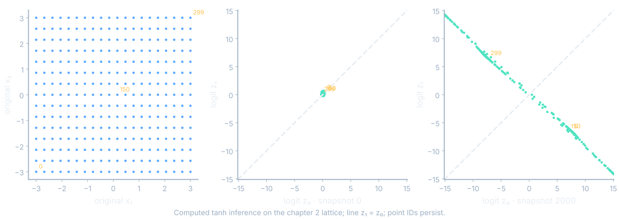
Follow one labeled lattice point between the two panels. Its identity stays the same; its coordinates change. In the final score plane, the decision is the straight line where the two logits are equal. Points above that line have the larger class-one score. Pull that comparison back through the network and it can form a curved boundary in the input plane.
The recorded tab preserves E3. Selecting an input point computes its logits from the latest available parameter snapshot and displays that snapshot’s step. A boundary picture may have been saved more recently. Both badges matter: a new boundary frame does not imply that an equally recent full parameter state was exported. The editable hand tab starts a separate calculation, with its own loss history and explicit initialization.
A small forward pass we can check
Let’s return to the small network from the forward pass. The input vector is (1,0). The first weight rows are (1,0), (0,1), and (1,−1); their biases are 0,1,−1. The two output rows are (1,−1,0) and (0,1,1), with zero output biases. These seventeen parameters are small enough to inspect together.
Every intermediate value
The first sums are 1×1+0×0+0=1, then 0×1+1×0+1=1, and finally 1×1+(−1)×0−1=0. Let t=(e²−1)/(e²+1), the exact expression for tanh(1). The hidden vector is (t,t,0). The output rows give t−t+0=0 and 0+t+0=t. Thus the logits are (0,t), and the probability of class one is exp(t)/(1+exp(t)). Its decimal value is 0.681699742195; the expression explains where that number came from.
For a general hidden layer, let the bold h denote its vector of current values, bold W its weight matrix, and bold b its bias vector. The subscript k identifies which layer we are applying. The next layer’s hidden values come from the same recipe:
$$\mathbf{h}_{k+1}=\tanh(\mathbf{W}_k\mathbf{h}_k+\mathbf{b}_k)$$In words: each hidden layer remixes the preceding values, shifts them, then bends them.
Replay the real run
Now we can look at training as changes in those parameters rather than a mysterious movement of a colored region. At initialization, E3 already has a boundary because its current weights already produce scores. Learning changes that boundary by repeatedly evaluating batches, computing derivatives, and updating the same parameter arrays. The split stays fixed through the replay.
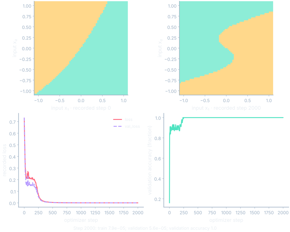
At step 2000, the saved training loss is 7.9e-05, validation loss is 5.6e-05, and validation accuracy is 1.0. The endpoint sources are media/runs/E3.summary.json#/values/final_loss, /values/final_val_loss, and /values/final_val_accuracy; their run pointers are the corresponding series entries at index 2000. These are measurements on the generated spiral and its recorded split.
Where this shows up when you train
A dense model is a useful starting point for a table of features because it can combine columns without assuming that neighboring columns are neighboring places. We still need the columns in a fixed order: swapping two features without swapping the corresponding weights changes the computation. The model knows which input slot it receives, not the human meaning of a CSV header.
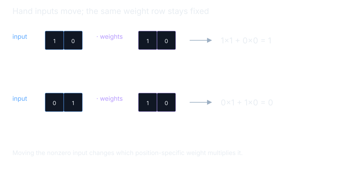
The hand failure is small enough to see immediately. A weight row (1,0) applied to input (1,0) gives 1×1+0×0=1. Move that nonzero entry to the other input slot, producing (0,1), and the same row gives 1×0+0×1=0. The pattern moved, but the position-specific rule did not move with it. A larger dense image classifier can learn several positions, yet it does not get a shared local rule automatically.
Keep the distinction between representation and optimization in view. Width and activation determine what transformations the model can express. The data, objective, learning rate, and update budget affect which transformation it reaches. A successful E3 run shows one combination working on one task. Other widths and rates in E9 are separate trials; selecting them in an interface cannot retroactively change the recorded E3 history.
What you now know
- Dense layers combine all preceding entries.
- The final class boundary compares the output scores.
- A recorded successful split does not establish performance on every input.
Where we’re headed
Convolution will share a local calculation so moving a pattern does not require an entirely different set of weights. Continue the story.