Keep every parameter in view
What exactly happens between an input and a model’s prediction? We will keep one small model fixed and follow every number. There will be no new weights hidden behind a diagram: the same seventeen parameters will return when we grade the prediction and calculate how to change them.
A class is a named output category. Binary classification chooses between two categories, which we will call class 0 and class 1. Our model receives two input numbers, produces three internal numbers, and then produces two class scores. A forward pass computes those outputs using the current parameters; it does not change the parameters.
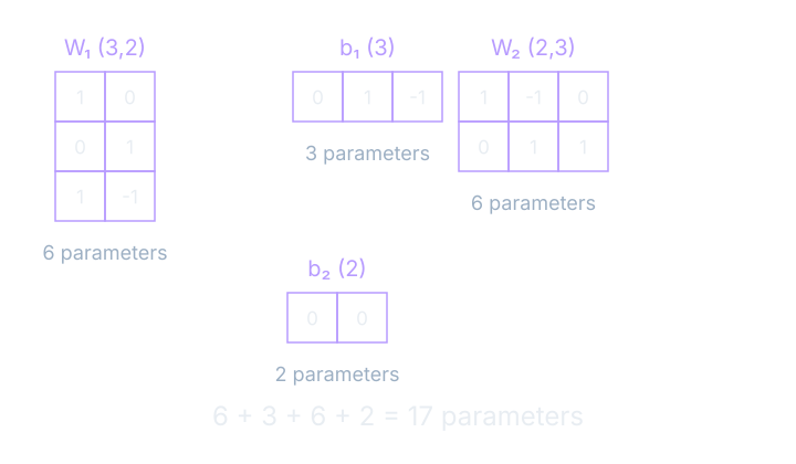
Here is the complete initial table, also stored in E2.json at snapshot 0. W₁=[[1,0],[0,1],[1,−1]], b₁=[0,1,−1], W₂=[[1,−1,0],[0,1,1]], and b₂=[0,0]. Subscript one names the hidden layer; subscript two names the output layer. There are twelve multiplying weights and five biases. The hidden activation is tanh, and the last layer is linear.
The model’s recipe matters alongside that table. A different activation would produce a different calculation using the same saved values. We also need the order of inputs and classes. Input position one matches the first column of W₁; output position zero names class 0. Those conventions keep the numbers attached to their intended roles.
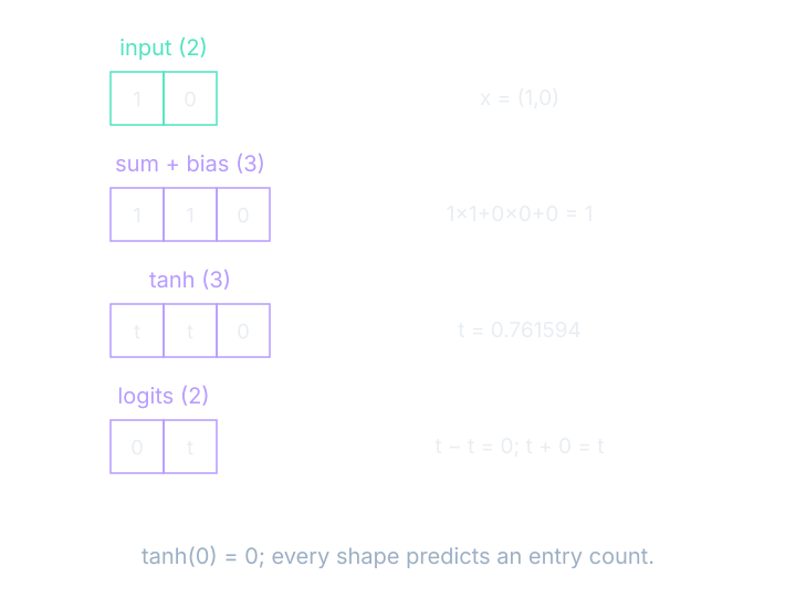
Begin with x=(1,0)
The hidden preactivation is the sum before the bend. Its first entry is 1×1+0×0+0=1. Its second is 0×1+1×0+1=1. Its third is 1×1−1×0−1=0. Together, the preactivation vector is (1,1,0).
The zero in the input makes several contributions vanish, but we still performed the complete row recipe. A different input could activate those contributions without changing the matrix. A zero input and a zero stored weight are different reasons for a product to be zero; retaining both values will matter when we compute derivatives.
A score is not yet a probability
A probability is a numerical share between zero and one for an outcome. A probability vector lists mutually exclusive outcomes whose shares sum to one. Softmax turns logits into such shares by exponentiating each score and dividing by the sum of all exponentials. Every class participates in that shared denominator.
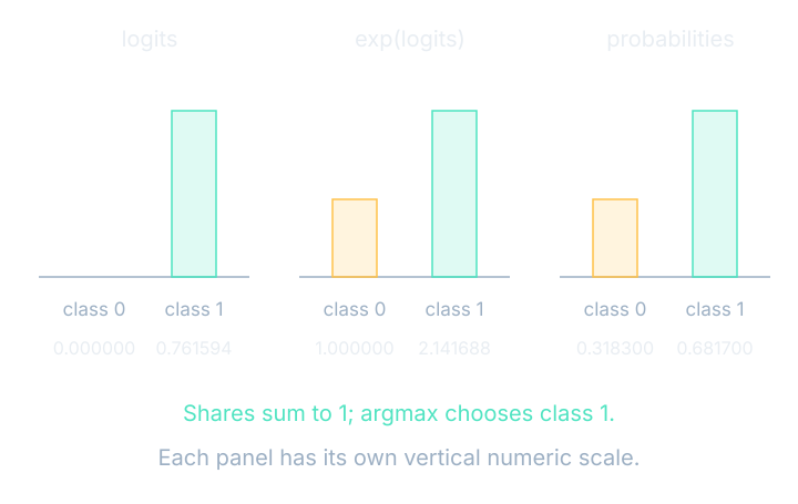
The exponential keeps every share positive for finite logits. A larger score produces a larger exponential and therefore a larger share. Dividing by the common total makes the shares sum to one. Notice the order of operations: exponentiating and dividing is different from dividing the raw scores by their sum, which would fail for many possible score vectors.
A probability share expresses the model’s assignment under this calculation. It is not automatically a statement that the model’s confidence is well calibrated on future data. We will later compare predictions with observed outcomes. Here the task is narrower: calculate the shares correctly from a fixed set of logits.
Softmax for the fixed model
The logits are (0,t). We have exp(0)=1 and exp(t)=2.14168768475. Their denominator is 3.14168768475. Dividing gives the probability vector (0.318300,0.681700), rounded to six decimals. Argmax means the index of the largest entry, so the decision rule chooses class 1.
For class index i, divide its exponential by the sum over all class indices j. The same denominator appears for every class. When one logit changes, the denominator changes too, so more than one probability share moves. That coupling will be part of the loss derivative we calculate later.
$$ \mathrm{softmax}(\mathbf{z})_i=\frac{e^{z_i}}{\sum_j e^{z_j}} $$In words: exponentiate each score, then divide by the sum so that the shares add to one.
For a separate arithmetic illustration, softmax on logits (2,1) gives (e/(e+1),1/(e+1))=(0.731059,0.268941). These are not the fixed model’s logits or probabilities. Subtracting 1 from both scores leaves the same shares because the common exponential factor cancels between each numerator and the denominator.
That cancellation gives a useful numerical procedure: subtract the largest score before exponentiating. The largest shifted score is then zero, avoiding unnecessarily large exponentials. The probabilities are mathematically unchanged. We retain full precision internally and round only the visible readout, so repeated use of rounded labels does not drive the computation.
Pause after every operation
Before advancing the interactive, predict which values should appear next. Start with the hidden products, then their sums and biases, then tanh. Each stage should use values that have already been computed. This is the same dependency picture we used to discuss parallel work, now attached to a complete numerical example.
See it move
The stepper expands one operation while keeping completed intermediate values available. At the end, compare its six-decimal probabilities with (0.318300,0.681700). Edit an input or parameter and follow the recalculated pass. Those changes create an edited hand example; they do not rewrite E2’s recorded initialization or its replay data.
Changing the second input is a useful probe because it is initially zero. It makes previously zero input-weight products visible. Changing a bias instead adds an offset regardless of the current input. Both operations can change the final probabilities, but their effects follow different paths through the same recipe.
Use the layer video’s wiring-to-matrix idea as a recap when it is available. The worked numbers on this page carry the complete pass independently: input, preactivation, hidden values, logits, and probabilities. If a result differs, compare those intermediate stages to locate the first disagreement rather than checking only the final class.
Where this shows up when you train
A prediction is the model output we use for a task. A decision rule such as argmax converts probability shares into a chosen label. Keeping those separate is useful when an application needs the probabilities themselves, a different decision threshold, or an explanation of why a marginal case received its label.
Save the complete table and input in mind: we will use x=(1,0), the same initial weights, and target class 1. Holding the example fixed lets us compare old and new losses meaningfully. If we changed both the model and the input between examples, we could not tell which change caused the difference.
What you now know
- A forward pass changes activations, not parameters.
- The fixed model produces logits (0,t) for this input.
- Softmax produces probability shares and argmax chooses a label.
Where we’re headed
Now we will supply the correct label and calculate how costly this prediction is. Continue to the next chapter.