The Graph Network (GNN)

What shape does it eat?

Suppose the important structure is who is connected to whom, rather than where a pixel sits or when a measurement arrived. Can we train a model that uses those relationships directly? We’ll begin with the same four-node contact star used in the sister book, then inspect a model trained on a recorded social graph.

A graph describes entities connected by relationships. A node is an entity; an edge is a connection between nodes. An adjacency matrix records which pairs are connected. Each node can also carry a feature vector. The graph drawing and these arrays describe the same connectivity, but the drawing’s horizontal and vertical positions need not be features supplied to the model.

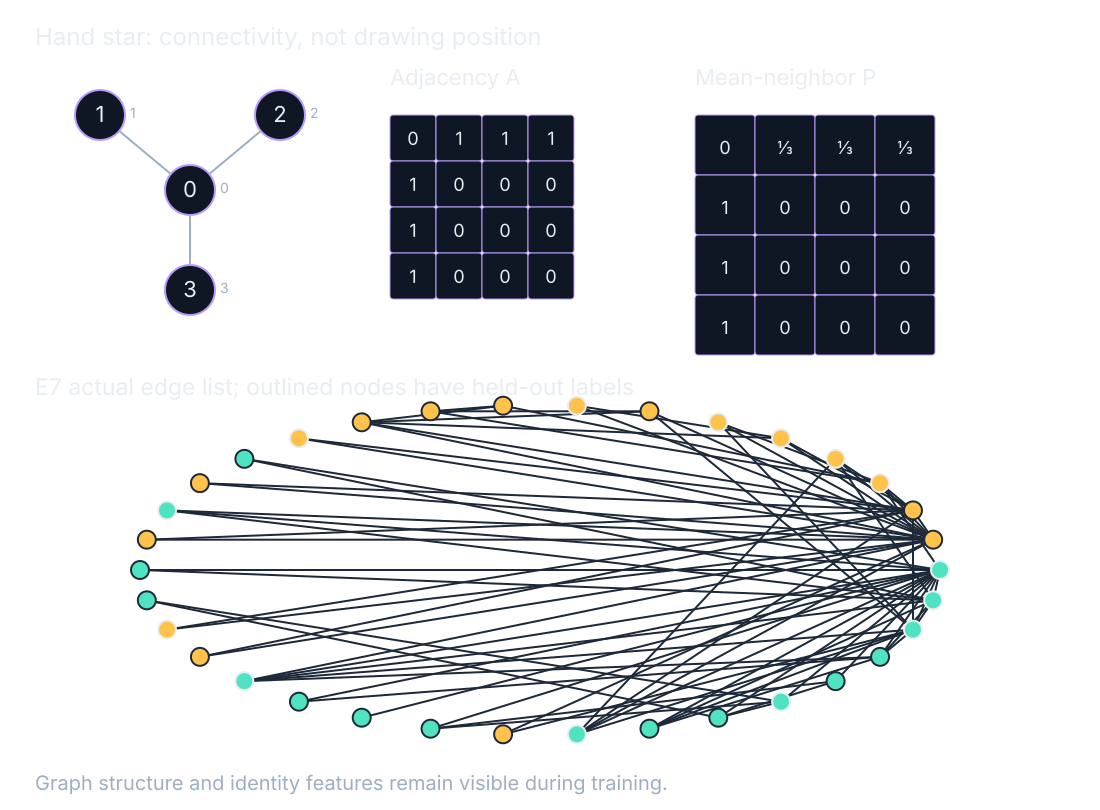
E7 uses the karate-club graph’s recorded edge list with identity node features: each node starts with its own coordinate marked. The task predicts a class per node. Training uses some labels, while other labels are held out. The graph structure and features remain visible. This is transductive evaluation, testing unseen labels on an observed graph. It is a different question from classifying nodes in an entirely new graph.

Let edges choose the neighbors

message passing gathers neighbor values, aggregates them, then updates a node. aggregation is a rule such as sum, mean, or max. permutation invariance means an aggregate remains unchanged when we reorder its inputs. Adding the neighbor values 1,2,3 gives the same total as adding 3,1,2. permutation equivariance means node outputs follow the same reordering as the corresponding input nodes.

Those properties let us change arbitrary node numbering without changing the represented problem. We must move adjacency rows and columns together with the corresponding features. Relabeling features alone would assign them to different entities. Dragging a node on the page changes only its display position. A model based on the given adjacency still gathers from the same neighbors after the drawing moves.

The same contact star, every update

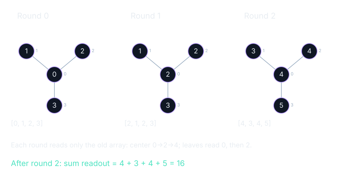
The hand star has center value 0 and leaf values 1,2,3. Its center connects to each leaf, with no edges between leaves. Our update keeps a node’s old value and adds the mean of its neighbors. Crucially, every node reads the old values from the same round. We do not let a leaf consume a center value that was already updated a moment earlier in the calculation.

For the first formula, bold H collects the node features, and bold I and P perform the hand keep-plus-mean update. E7 uses a different gather rule. Its A is the original adjacency, I adds self-connections, and d counts each node’s connections after that addition. A hat marks the normalized adjacency. Bold W and b are the learned weights and biases. We write all three operations so the toy and trained rules remain distinguishable:

In words: keep the node’s old feature and add its neighbors’ mean.

In words: add self-connections, then scale each connection by the square root of the two endpoint degrees.

In words: gather normalized neighbor features, transform them with the learned weight matrix, add bias, and apply the activation. The superscript top transposes the weight matrix: it swaps rows and columns without changing entries. Stored weights are output rows by input columns, as in chapter 3; the transpose lets these row-shaped node features multiply them.

Replay predictions on the observed graph

The first E7 layer maps 34 identity features to four hidden coordinates. Its weights and biases contribute 4×34+4=140 parameters. The second maps four coordinates to two scores, contributing 2×4+2=10. The model therefore has 150 trainable parameters. The normalized adjacency is part of its fixed graph computation rather than another trainable weight table.

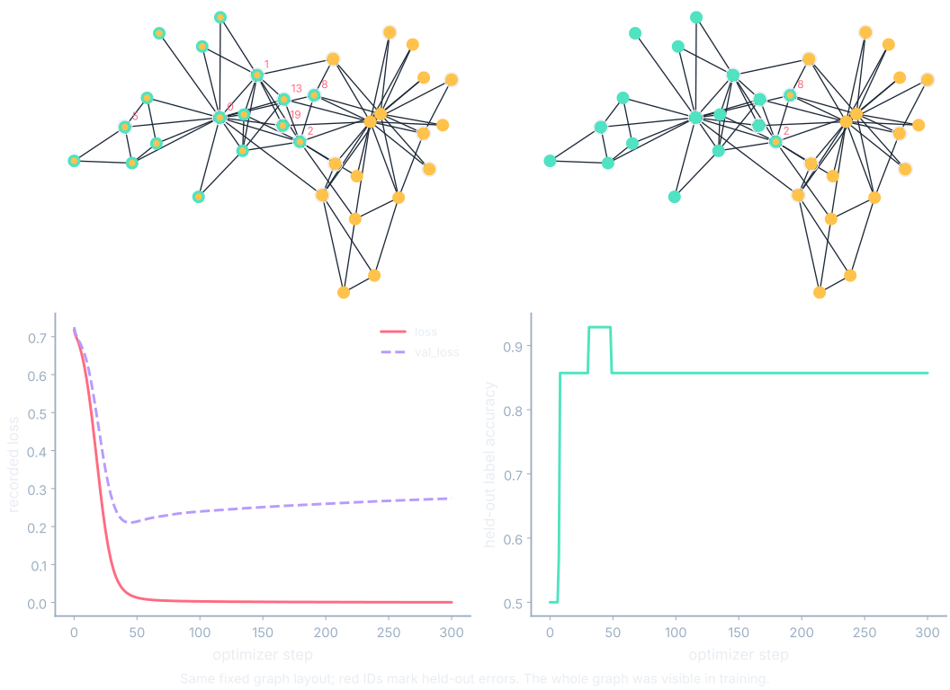
At step 300, training loss is 0.000525, validation loss is 0.273955, and validation accuracy is 0.857143. These values come from media/runs/E7.summary.json#/values/final_loss, /values/final_val_loss, and /values/final_val_accuracy, with corresponding run-series pointers at index 300. The difference between training and validation loss is visible alongside the graph. The held-out nodes deserve attention even when most training labels are predicted confidently.

Where this shows up when you train

Contact networks and road connectivity offer relationships that can guide a gather rule. A table of unrelated records does not acquire useful edges because a graph model is available. We need a reason why each connection should help answer the task. If distance or direction matters, those quantities must enter the representation explicitly; they are not supplied by dragging the diagram into an attractive layout.

Mean aggregation loses information about how many neighbors contributed: repeated equal values have the same mean. Sum retains that count but can grow with neighborhood size. Max keeps a strongest value while discarding the rest. These are concrete information choices. Before stacking more message rounds, inspect what one round preserves, what it loses, and how far a signal can travel along actual edges. A deeper graph model cannot recover a distinction already erased by its inputs or aggregation rule.

Where we’re headed

An autoencoder will learn a compact representation by trying to reconstruct its input. Continue the story.