The Autoencoder

What shape does it eat?

What if the answer we ask a model to produce is its own input, but we force the information through a narrow passage first? Copying every entry directly would be easy. Reconstructing it from fewer numbers makes the model choose what to preserve. We can inspect that choice with the same matrix arithmetic and training records used for classification.

An autoencoder is trained to reconstruct its input. The encoder maps an input into a compact representation, a set of numbers used by the next computation. The latent is the internal representation supplied to the decoder, which maps it back to the output shape. A bottleneck restricts the representation’s width or information capacity. reconstruction loss scores the difference between the original input and the reconstruction.

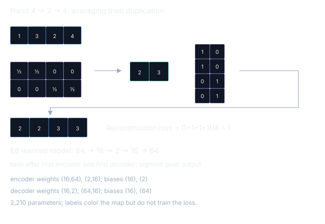
E8 takes flattened 8×8 digit pixels, so one input has 64 entries. Its encoder maps 64→16 with tanh, then 16→2 with a linear layer. Its decoder maps 2→16 with tanh, then 16→64 with sigmoid pixel outputs. The target is the original pixel vector. Digit labels color the displayed map; they do not enter the reconstruction objective. This task is self-supervised because the data supplies its own target.

The target is the input

The target matches the input, so a useful solution must preserve information that helps reconstruct many examples. The decoder learns how to turn nearby latent coordinates into output vectors. That does not guarantee that distances in the latent plane match distances between original images, or that one direction has a convenient human meaning. Those are properties to inspect rather than assume.

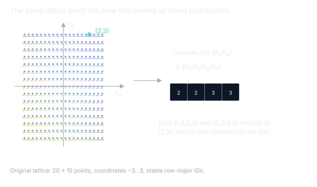
The hand lattice reuses the coordinate identities from space that stretches. We can decode each point instead of treating the plane as an abstract scatterplot. With our hand decoder, latent (h₁,h₂) becomes (h₁,h₁,h₂,h₂). Moving horizontally changes the first pair of output entries; moving vertically changes the second pair. The learned E8 decoder has a more complicated mapping, but it still produces a definite vector for each selected latent point.

Encode, decode and measure what was lost

Use input x=(1,3,2,4). Our hand encoder averages adjacent pairs with rows [1/2,1/2,0,0] and [0,0,1/2,1/2]. The bias is zero and there is no nonlinear bend. The decoder rows are [1,0],[1,0],[0,1],[0,1]. This entire toy is linear, which lets us identify exactly what information is discarded.

Bold x denotes the original vector, bold h the latent, and x with a hat the reconstruction. The count n is the number of input entries over which we average. The encoder and decoder stand for the actual sequences of operations, including any activations:

In words: compress the input, reconstruct it, then average its squared pixel errors.

Replay the learned representation

E8 learns both mappings together using the pixel loss. The class labels are absent from that optimization, so the model has no direct instruction to separate every digit class in the latent plane. A cluster may still emerge because related images share reconstructible structure. The correct next action is to inspect the saved coordinates and reconstructions, not assign a meaning to each axis from the picture alone.

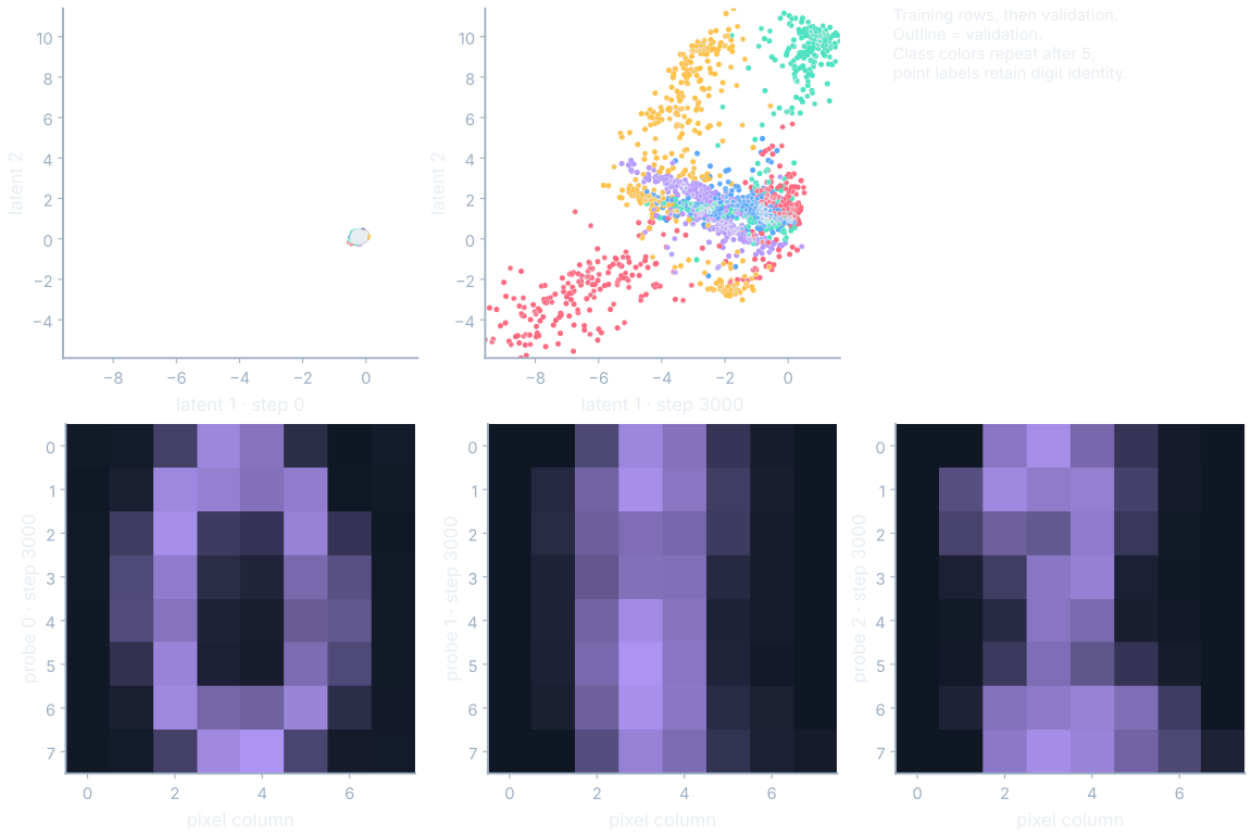
At step 3000, E8 has training loss 0.038305 and held-out reconstruction loss 0.040935. They come from media/runs/E8.summary.json#/values/final_loss and /values/final_val_loss, pointing to the corresponding series values at index 3000. These are mean squared pixel reconstruction errors. They are not classification accuracy, and multiplying one by a hundred does not turn it into a percentage of correctly recognized digits.

Where this shows up when you train

A reconstruction can look broadly recognizable while losing contrast in particular pixels. We should inspect the differences at the same locations, not rely on a general impression of similarity. The figure compares the saved probe originals with their final reconstructions and highlights the largest mean error among those recorded probes. That selection is limited to the available probes; it does not identify the worst image in the full dataset.

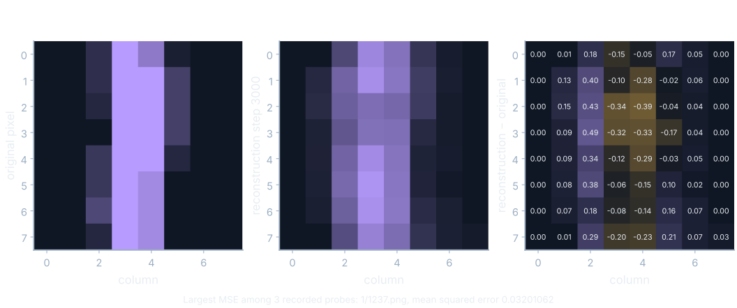
The original pixels come from the shipped PNG files using the stored training-order mapping: for each fixed digit label, choose its first training example. Another image with the same digit label would not be the same probe. The residual grid subtracts those original values from the saved reconstruction values, letting us identify both positive and negative errors. Compare a bright residual cell to the corresponding original and reconstructed pixel before describing lost detail.

For a new dataset, choose preprocessing, a reconstruction objective, and an independent evaluation set before judging the latent picture. Preserve the original scale so a pixel difference has a clear meaning. If the eventual task is classification or anomaly review, evaluate that task explicitly as well. The compact plane is a useful place to inspect behavior, while the saved arrays and stated objective keep the inspection tied to checkable numbers.

Where we’re headed

The model recipes are now visible. We will turn real files into their required shapes without leaking evaluation information. Continue the story.