Reading the Graphs: What Training Should Look Like

The four curves

The loss is falling, but the saved best model is six epochs old. Is training still helping? We can answer only after naming what each curve measures. Let’s read four curves from our weather-model recordings, keeping the task’s score beside the error that training tries to reduce.

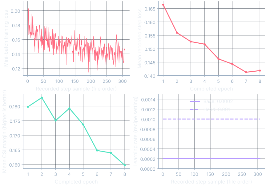
Training loss per step is one mini-batch’s error. Training loss per epoch normally averages a whole pass, weighting batches by their sizes when necessary. These files sample steps sparsely, so our epoch training curve is explicitly the mean recorded step loss. It cannot recover an exact whole-pass average.

A validation score measures performance on held-out examples the model does not fit during its parameter updates. The learning rate is a recipe setting, not a measurement of the model. We plot it to see when the update scale changed. Keep the loop’s batch, epoch, and schedule vocabulary and loss units in view.

The band and the level

Each mini-batch contains different examples. Some are harder, so its loss can rise even while the run improves over many updates. Read the height of the band across an interval before interpreting one wiggle. Sampling noise is variation from which examples were selected; the changing parameters can contribute variation too.

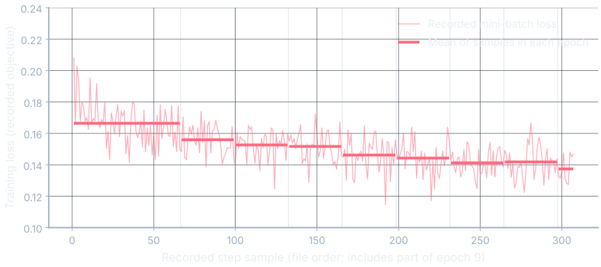
The horizontal coordinate counts recorded samples, not optimizer updates or elapsed seconds. This capture has completed evaluations for epochs 1–8 and ten additional step samples from epoch 9. We retain those samples in the trace without inventing a ninth validation point. The at-home exercise below explains which related curve trainkit actually records.

From scratch and from a checkpoint

A fine-tune starts from learned weights. The v2 run started from scratch; Alaska continued from its checkpoint. Their architecture has 27,223,297 parameters. A fine-tune can begin near the earlier run’s finishing loss, leaving less distance to travel, but a different regional dataset can change the starting difficulty.

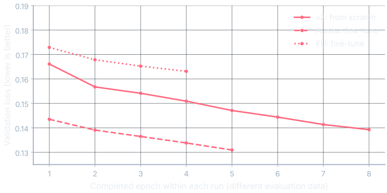
Validation loss is the error objective on held-out examples. Displayed to six decimal places, v2 moves from 0.166102 to 0.139279 over eight completed epochs; Alaska moves from 0.143522 to 0.130958 over five. Alaska starts close to v2’s ending level. This comparison describes shape, not a controlled ranking across datasets.

The loss falls while the score stalls

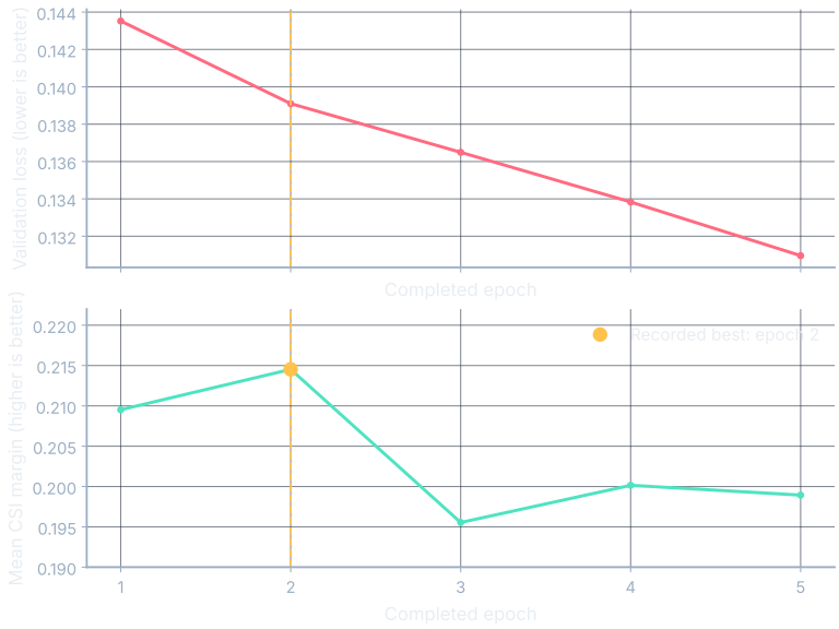
A plateau here means an interval without a new best task score. It need not be a perfectly horizontal line. Alaska’s score peaks at epoch 2, then moves below that peak while validation loss keeps falling through epoch 5.

The loss proxy improving does not mean the thing we care about is still improving. This is different from training loss falling while validation loss rises. Alaska’s validation loss also falls. When It Goes Wrong separates diagnostic symptoms; this curve alone does not establish overfitting or its cause.

Read the recipe beside the result

Both v2 and Alaska record constant learning rates: 0.0002 for the base parameter group and 0.001 for the output head, five times as large. A parameter group is a set of weights assigned the same optimizer settings. There is no warm-up ramp or scheduled drop hidden in these traces.

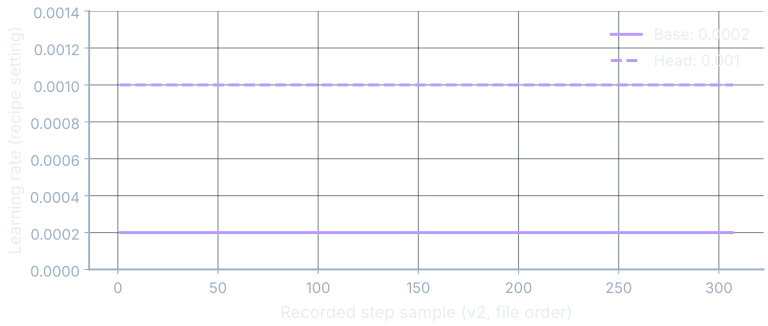
The loop’s constructed step and warm-up sketches show the other shapes. A step schedule drops at a chosen point; warm-up ramps upward initially. Either changes the update recipe and may change the loss trend or its variability. Neither guarantees a visible kink. The dashboard’s constructed schedule example continues that distinction without presenting an invented weather run.

Steady, spiking, or pinned at the ceiling?

A gradient norm measures gradient magnitude. A steady trace stays in a relatively narrow range; occasional spikes depart from it. A trace pinned at a clipping ceiling repeatedly reaches the imposed cap. These shapes call for different checks.

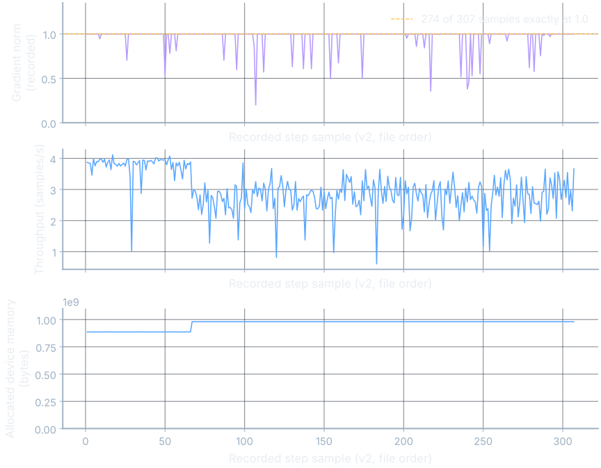
Exactly 274 of 307 recorded norms equal 1.0: 89% at whole-percent precision. The minimum is 0.1993151158094406. Clipping limits the gradient supplied to the optimizer, so repeated contact with the ceiling deserves inspection. It does not show how far the unmodified gradients exceeded the cap, and an adaptive optimizer’s actual parameter movement cannot be reconstructed from this norm alone.

Throughput, utilization, and memory

V2’s throughput ranges from 0.6071397294084898 to 4.11412364649941 samples per second. The same model can process examples at quite different observed rates. Waiting for data, evaluation, and checkpoint work are possibilities to investigate. The capture does not isolate their contributions or record GPU utilization, so it cannot establish that this run was loader-bound.

Allocated device memory ranges from 885,530,112 to 980,466,688 bytes: a near-plateau on the panel’s zero-based scale. This sampled allocation excludes temporary peaks. V2’s run metadata says two workers; its first epoch records one and epochs 2–8 record two. The steps identify device cuda:0, so we do not interpret this trace as aggregate usage of two GPUs.

Patience and the recorded best

Patience is how many evaluations without a new best we allow before stopping. These files record a plateau counter, not a verified stopping configuration. V2’s counters are 0,0,1,2,3,4,5,6; Alaska’s are 0,0,1,2,3.

V2’s epoch-2 score is 0.18292, displayed to five decimals. Epoch 3 drops to 0.17505; epoch 4 partially rebounds to 0.17924, still below the peak. The counter never resets after epoch 2. Its best checkpoint remains epoch 2 even though validation loss falls for six more epochs. The latest state and the saved best answer different requests.

Lay every retained epoch on the same axes

The super-resolution model, which reconstructs a finer image, gives us a quieter late-stage example. These are the five most recently retained epochs of a longer run, after its loss function changed. They are numbered 11–15. The model has 1,367,553 parameters; the file does not contain its earlier training history.

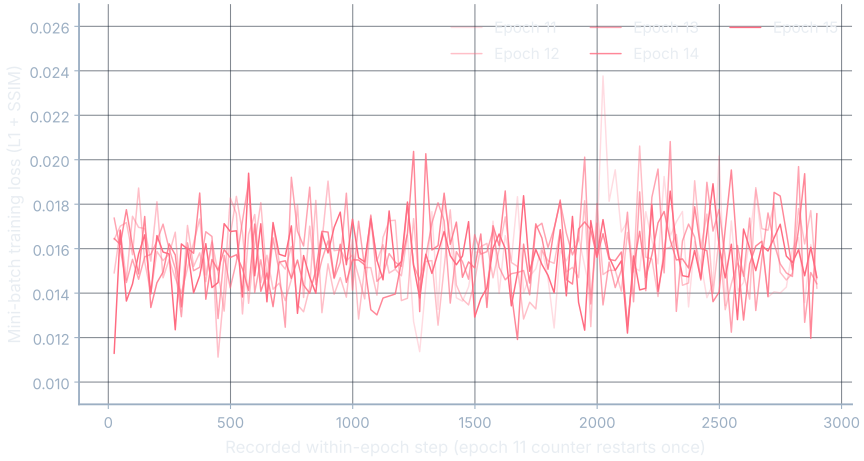
run.json records a change at epoch 11 from absolute-error loss to absolute error plus structural similarity, which compares local brightness, contrast, and structure. The recorded epoch loss changes from 0.015799845840782215 at 11 to 0.015746532272849445 at 15. Older lines are fainter; their transparency represents age, not confidence.

Where this shows up when you train

Choose the evaluation measure before interpreting progress. Then identify the data split, averaging rule, and best-checkpoint flag. The widget starts at Alaska’s first evaluation. Scrub the visible history and choose “Stop here” before revealing the later epochs and recorded best. Repeat with v2 and compare the result.

See it move

Run this yourself

Where we’re headed

We can now read the main curve shapes. Next we will connect them with internal model measurements at a shared progress point. Continue to the next chapter.