Super-Resolution, 2×

The problem

A cloud edge looks blocky when its source pixels cover a large patch of ground. Enlarging the picture fills more display pixels, but it does not create new measurements. super-resolution learns a finer image from a coarser one. We will ask what it adds beyond an interpolation method we can already run without training.

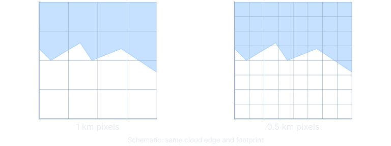
The visible-band task described here brings coarser bands toward the red band’s finer sampling. The earlier runs include another scale, so we will keep each run’s scale and band attached to its score. Combining them into one generic “resolution gain” would make the result easier to advertise and harder to interpret. Source §2.

The data

A training example degrades an observed band and asks the model to restore it. There is no measured finer blue-band truth: this is a proxy task. In the selected blue probe, the observed 1 km band supplies HR and its box-averaged 2 km version supplies LR. Source §7. The target is the image we withheld from the model’s input, not a sharpened version of its own answer. The intended scale-2 tensor pair is (1, 64, 64) → (1, 128, 128). Earlier scale-4 evaluation used 64→256 spatial dimensions. Source §2.

The Himawari red training summary records 41,400 training and 3,600 validation sequences across 6 held-out scan days. Its parameter count belongs to a scale-4 run: 1,515,265. The scale-2 sr-v3b-blue model has 1,367,553 parameters. We do not attach either count to an unspecified scale. Source §2.

The model

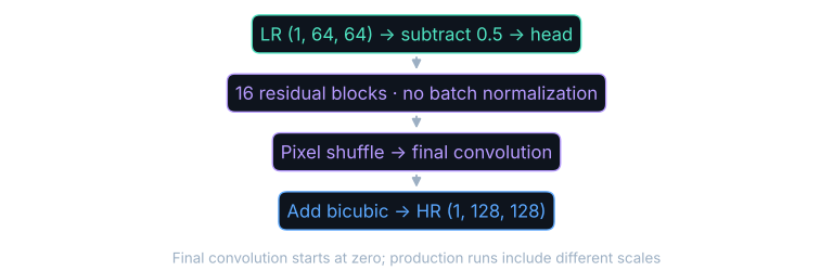
bicubic interpolation estimates intermediate values by a fixed local calculation. residual learning trains a correction to that baseline. The baseline already handles much of the smooth structure, so the network can concentrate on differences. We reuse shared local filters rather than re-teaching them here.

pixel shuffle moves channel entries into finer spatial positions. It rearranges learned features rather than looking up missing observations. With the final convolution zero-initialized, the correction starts at zero, so the complete output initially equals bicubic. Subsequent updates can help or hurt; the initialization does not guarantee every later checkpoint beats the baseline. Source §2.

Where this comes from

The architecture is not novel: Lim et al.’s EDSR (2017) follows Dong et al.’s SRCNN (2016, TPAMI); Zhang et al.’s RCAN (2018) adds channel attention. Satellite-band super-resolution is already explored: White et al. (2024, AIES) use degrade-and-restore training on GOES-16 ABI bands. We found no dedicated peer-reviewed Himawari AHI super-resolution paper. Ours is the Himawari band corpus, loss-weight sweep, and blind pairwise judging protocol. Source §6.

The loss and why that loss

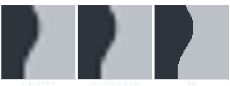
PSNR measures squared pixel disagreement. For peak value P and mean squared error M, $\mathrm{PSNR}=10\log_{10}(P^2/M)$ dB. With normalized, bounded pixels it runs from zero to infinity; an exact match has infinite score. Blue’s 39.758 dB versus bicubic 38.664 dB means smaller squared error, a gain of 1.094 dB. No interval was measured, so the sampled gain does not establish reliability across new scans. PSNR rewards blur; we also track structural similarity and blind human choices. Source §2.

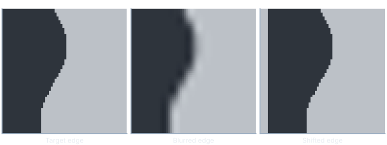
SSIM compares brightness, contrast, and how local patterns vary together. In one line, $\mathrm{SSIM}=\mathrm{brightness\ agreement}\times\mathrm{contrast\ agreement}\times\mathrm{structure\ agreement}$, with range −1 to 1 and 1 an identical match. Probe 2010’s 0.9660 versus bicubic 0.9500 means closer local structural agreement, not 96.6 percent correct pixels. Neither has a confidence interval; this selected crop cannot establish a general winner. SSIM depends on its local windows and can miss convincing but false detail, so we retain the target comparison and blind judging. Source §7.

In words: add absolute pixel error to half the structural-similarity shortfall.

The masked loss excludes invalid night and limb pixels. Structural comparisons use valid windows. Both model and bicubic must see the same target, mask, and scale. Source §2.

Training as it actually ran

The Himawari red run used batch size 17, constant learning rate 2e-4, half-precision autocasting, and 8 epochs. The run summary reports 3.25 hours and 6.8 minutes per epoch as separate summaries. We do not multiply one into an explanation of the other; the retained timing labels do not establish that relationship. Source §2.

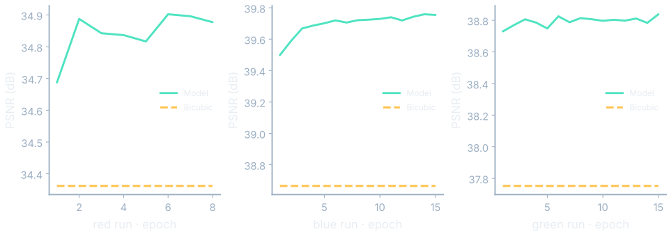
At the selected epochs, red reaches 34.902 versus 34.362 dB at epoch 6; blue reaches 39.758 versus 38.664 at epoch 14; green reaches 38.838 versus 37.752 at epoch 15. The run summary reports the corresponding gains as +0.541, +1.094, and +1.086 dB. Reported gains use underlying precision, so rounded endpoints need not subtract exactly. Source §2.

Outputs

A brightness stretch changes appearance without changing stored reflectance. If each panel were stretched separately, darker model output could look just as bright as the target. The shared stretch keeps that display adjustment from hiding a prediction error.

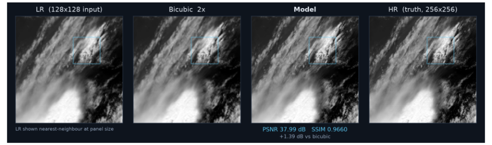
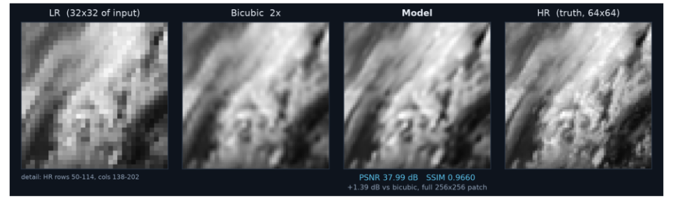
See it move: use the magnifier to inspect a cloud edge, then switch between bicubic, the learned correction, and the observed proxy target. The flipbook below keeps the same blue-band probe identity across epochs. Its PSNR label comes from the held-out score table, not a fresh calculation on the visible tile.

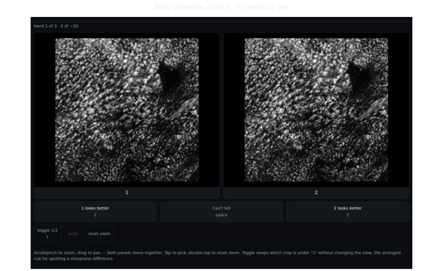
The picture asks a judge to choose between anonymous crops. The Bradley–Terry model converts such choices into relative strengths: $p(A\text{ beats }B)=e^{s_A}/(e^{s_A}+e^{s_B})$, between zero and one. The strength scores s have no absolute scale; only their differences matter. We have no usable human verdicts, no model or bicubic judge score, and no uncertainty interval to read aloud. A pooled winner would be invented. Preferences can reward attractive false texture, so the observed target, PSNR, and SSIM remain alongside the blind test. Bradley and Terry (1952) Source §2.

What it is not

An interpolation baseline is also a debugging tool: the untrained residual network should reproduce it exactly on the same input.

A paired evaluation keeps the reconstruction method accountable to observations rather than visual plausibility alone. Bicubic remains useful after training: it is the starting prediction, the comparison baseline, and the quantity to which the residual is added. Keep all of those roles clear. If the learned correction creates an artifact, the baseline provides a concrete reference for identifying what the network changed.

Where this shows up when you train

Inspect both the task score and the kind of error a user notices. The reported gains are modest and the model cannot invent sub-pixel truth. Night pixels are masked from this evaluation. A daytime score should not silently become a claim about an all-hours product. Source §2.

Run this yourself

trainkit upscale samples/tile.png --output upscale-output

The command writes run.json and model.json. Add --dry-run to preview the replacement targets. Keep your output separate from the bundled book artifacts. The run records the data shapes, split, objective, baseline, model score, and elapsed time; the model export contains the actual learned weights.

Repeat the run before changing the recipe. Then change a single input or model choice and compare on the same held-out examples. A different random split can change a score even when the learning rule is unchanged. Keeping the original baseline makes it possible to distinguish an improvement in the learner from an easier evaluation problem.

Where we’re headed

Next we will carry the same questions into Nowcasting the Radar.